Manning’s n Calibration - Example 24

When using HEC-RAS, the users objective is to create a model that is accurate and properly represents a real-world river system. However, there are some features of the river that are not explicit but must be determined by trial and error and sound engineering judgment. If the river has reliable gages, for unsteady flow models, the user can use the historic gage flows to calibrate the model to real-world events. One of the primary inputs that is adjusted during calibration is the Manning's n value since this variable often has the most uncertainty and variability amongst the HEC-RAS input. Since calibrating a model (especially a large one) to one or more gages can be a long and tedious task, HEC-RAS has a feature that will automate the calibration of the Manning's n values. This example will demonstrate how to use this feature. The model used in this example is a portion of the Mississippi River and the Ohio River at their confluence. While the data is from actual studies, the models and results of this example application do not represent current or future conditions of the system.

To review the data files for this example, from the main HEC-RAS window, select File and then Open Project. Go to the directory in which you have installed the HEC-RAS example data sets. From the "Applications Guide\Chapter 24 – Mannings n Calibration" subdirectory, select project titled "Manning's n Calibration." Once opened, this will activate the following files:

Plan: "Automatic Calibration"
Geometry:"Mississippi Ohio Junction"
Flow: "Mississippi Ohio"

Example 24 - Mannings-n-Calibration.zip

Geometric Data

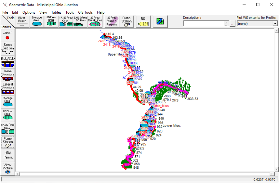
To view the geometric data for the river system, from the main program window select Edit and then Geometric Data. This will activate the Geometric Data Editor and display the river system schematic as shown in the figure below. The schematic gives a visual representation of the geometric elements entered by the user.

Cross Section Data

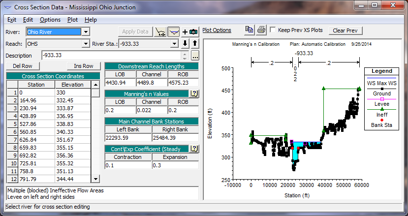
The cross section data consists of the X-Y coordinates, Manning's n values, contraction and expansion coefficients, etc. The user can view this data for each river station by selecting the Cross Section icon on the left side of the Geometric Data Editor. All the data for each cross section was manually entered, an example of which can be seen in the figure below. Levees and ineffective flow areas were added to some of the cross sections. These features are accessed under Options of the Cross Section Data Editor. Look to Chapter 6 of the User's Manual for more information on entering cross section data.

Stream Junction Data

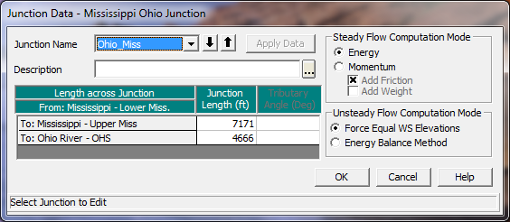
Once a junction was established by connecting reaches on the river schematic, junction data was added by clicking on the Junct icon from the left side of the Geometric Data Editor. This activated the Junction Data Editor as shown in the figure below. This model contains one junction that uses the Energy method for steady flow computations and Force Equal WS Elevations for unsteady flow computations.

Creating Storage Areas

When creating the storage areas, first the Storage Area icon was selected from the Tools toolbar (not to be confused with the Storage Area icon from the Editors toolbar) of the Geometric Data Editor. The pointer was then placed at the desired location on the river schematic and the storage area was drawn by single clicking and dragging the mouse for each desired point for the storage area. The final point for the storage area was selected by double clicking the mouse. Upon double clicking the mouse, a dialog box appears requesting a storage area name. A name was entered for each storage area created. Points on a storage area may be added or removed by using the Add Points to a Reach or SA and Remove Points to a Reach or SA options found in the Edit menu.

Entering Data for a Storage Area

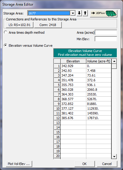
After the storage area was drawn in the Geometric Data Editor the elevation volume relationship for the storage was established. The data was entered in the Storage Area Editor, displayed in the figure below, which is opened by selecting the Storage Area icon on the Editors toolbar. All the storage areas in this example used the Elevation versus Volume Curve to determine a relationship for calculating storage area. This method was selected by clicking the corresponding radio button and then filling in the elevation volume table listed below it (see figure below).

Storage Area Connections

Storage area connections are used to connect storage areas to other storage areas. In this example elevated roadways that divide storage areas are modeled as storage area connections. This feature is used by first selecting the SA/2D Area Connection icon from the Tools toolbar in the Geometric Data Editor. A line can be drawn from one storage area to another by right clicking on the first storage area and then double clicking on the second. A prompt comes up that will ask for the name of the connection. After the user enters a name for the SA connection, it can be selected and edited from the SA/2D Area Connection Editor, which is located on the Geometric Data Editor (above).

The storage areas that the connector transferred water to and from were selected by pressing the Set SA buttons next to the From and To location fields. For this example, the Structure Type was chosen as Weir from the drop down menu for all of the storage area connections. The figure below shows the Connection Data Editor when illustrating the Weir structure types.

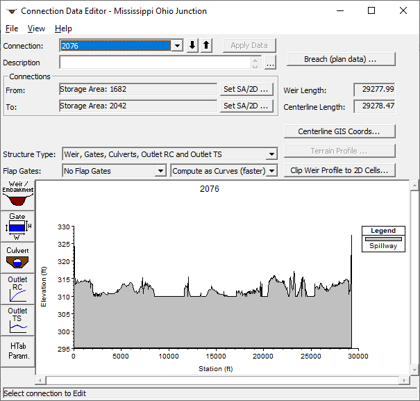
Lateral Structures

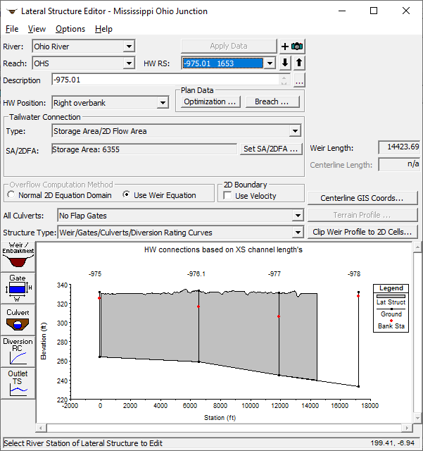
A lateral structure was placed at several river stations throughout the system. This was accomplished by selecting the Lateral Structure icon from the Editors toolbar in the Geometric Data Editor. After selecting the icon, the Lateral Structure Data Editor appears, as shown in the figure below. Once the proper reach and river were selected, under the Options menu, Add a Lateral Structure was selected. HEC-RAS then prompts the user to enter the location of the structure. This placed the beginning of the structure between the cross section river station immediately upstream of the lateral structure river station and the cross section river station immediately downstream of it. The All Culverts and Structure Type fields were left at their default selections of No Flap Gates and Weir/Gates/Culverts/Diversion Rating Curves for all of the lateral structures in the system.

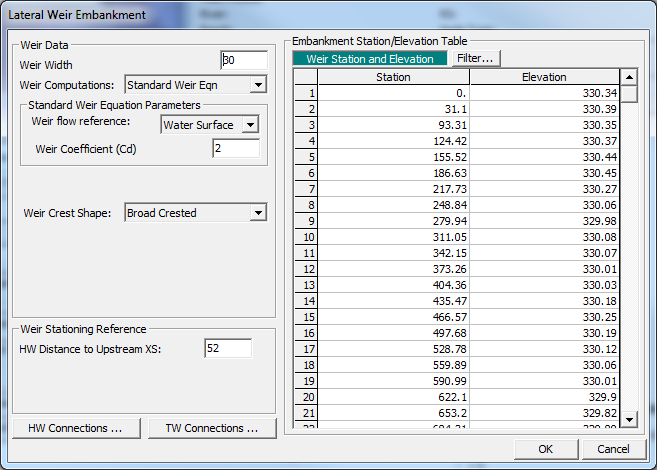
To enter weir data for the structure, the Weir/Embankment icon was selected from the Lateral Structure Data Editor. The data were entered as shown in the figure below on the Lateral Weir Embankment Window. The editor requires an entry for the following fields: Weir Width, Weir Computations, Weir flow reference, Weir Coefficient, Weir Crest Shape, HW Distance to Upstream XS, and TW flow goes. Further description of these fields can be found in Chapter 6 of the User's Manual.

Returning to the Lateral Structure Data Editor, the HW Position was selected as either "Left overbank" or "Right overbank" from the pull-down menu depending on where the lateral structure resided. The Tailwater Connection Type was chosen as Storage Area, meaning that the lateral structure connected the river to a storage area, or Out of System, which means that the water leaving the river via the lateral structure is no longer modeled upon leaving. For the Storage Area type tailwater connections, an individual storage area was selected to correspond to the lateral structure by clicking the Set SA/2DFA button. A window then popped up allowing the user to select a storage area to connect to from a pull-down menu.

Inline Structure

For this example there were only two inline structures, both of which were on the Ohio River. To add an inline structure, the Inline Structure icon was selected from the left side of the Geometric Data Editor. This activated the Inline Structure Data Editor as shown in the figure below. Ohio River was chosen as the river, then, Options and Add an Inline Structure were selected and the river station was entered as the location for the weir. The schematic then displayed the cross section data for the river station immediately upstream of the weir location.

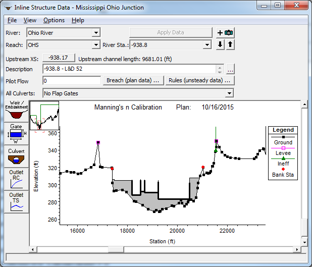
Next the weir data was entered. To enter the data for the weir, the Weir/Embankment icon was selected from the left side of the Inline Structure Data Editor. This activated the Inline Structure Weir Station Elevation Data Editor as shown in the figure below. This editor is similar to the deck/roadway editor used for bridges and culverts.

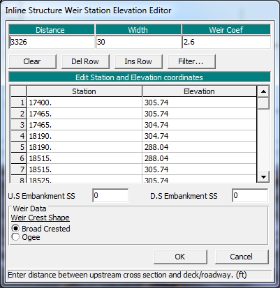
The top row of the editor consists of three data entry fields. For the first field, the user must enter the Distance from the upstream cross section to the upstream side of the weir. Next, the Width of the weir was entered (both inline weirs has a width of 30 feet). The last field in the top row of the editor is the Weir Coefficient and was entered as 2.6 for both inline weirs, coinciding with the Broad Crested weir shape chosen at the bottom of the editor.
The central portion of the editor consists of a table in which the user must enter the station and elevation data for the weir. With these weir stations and elevation, the program will block out the entire area below the weir crest.

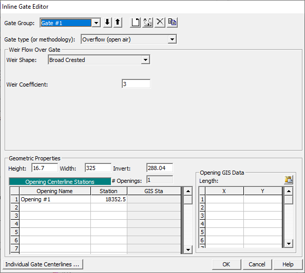
To enter the data for the gates, the Gate icon was selected from the Inline Structure Data Editor (above). This activated the Gate Editor as shown in the figure below. Each inline structure had four gates, with each gate belonging to its own gate group. A separate gate group for each gate was created by clicking the New Gate Group button (looks like a blank sheet of paper at the top of the editor). The Gate type (or methodology) was changed to Overflow (open air) from the pull down menu for all gates. The Weir Shape was selected as Broad Crested Weir and the Weir Coefficient was entered as 3. Each gate's geometric properties were entered on the left side of the editor (see figure below). The OK button was selected at the bottom of the Gate Editor and the gates appeared on the Inline Structure Data Editor as shown in the figure below. The Inline Structure Data Editor was then closed.

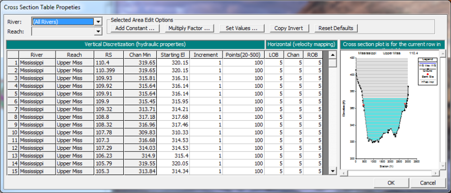
Cross Section Table Parameters

In HEC-RAS, cross sections are processed into tables of elevation versus hydraulic properties of areas, conveyances, and storage. The user is required to set an interval for spacing the points in the cross-section tables. In the Geometric Data Editor the icon Htab Parameters was selected under the Editors toolbar. This displays the Cross Section Table Parameters Window shown in the figure below. The starting elevation, table increment, and number of points columns are automatically filled by the program but may be changed by the user. The program automatically starts the table for each cross section one foot above the channel invert. The program chooses a table increment and number of points by first attempting to use 20 points, and choosing an increment that will put the table up to the top of the cross section. If this results in too large of an increment (greater than 1.0 foot) the program will use a one foot increment and add additional points to get the table to the top of the cross section. In this example, since the Mississippi River and Ohio River are very large rivers that have significant variations in stage, the maximum number of points (500) had to be used and the increment was greater than 1.0 at some river stations. The user can set individual values for each cross section if it is deemed necessary. Warning: Always ensure that your cross section tables encompass the complete range of stages that will be modeled. If the tables do not go up to a high enough elevation, the program will have to extrapolate during the computations. More often than not, the extrapolation causes instabilities in the results. To visualize the extent of the tables, a graphic of individual cross sections is shown on the right hand side of the window. The graphic displays the cross section corresponding to the row in which you cursor lies in the table.

Unsteady Flow Data

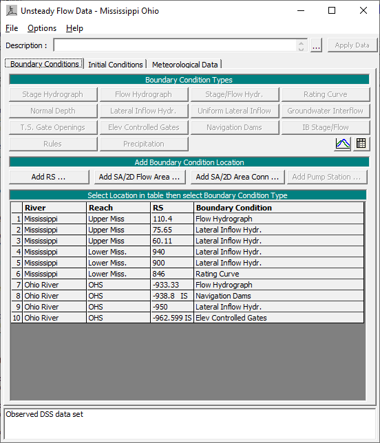
The user is required to enter boundary conditions and initial conditions for the system at the beginning of the simulation period. For additional information on unsteady flow data refer to Chapter 8 of the User's Manual, Performing an Unsteady Flow Analysis. The Unsteady Flow Data Editor, shown in the figure below, was selected from the main program window under the Edit menu.

Boundary Conditions

Boundary conditions are required for the farthest upstream and downstream cross sections of the river system. Upon entering the Unsteady Flow Data Editor the farthest upstream and downstream cross sections will automatically be located in the boundary conditions column. In addition, features such as gated inline structures, which also require a boundary condition, will automatically be populated in the Boundary Condition table. In this example there are 10 total boundary conditions: two upstream BC, one downstream BC, and seven internal BC.
Boundary conditions are set by highlighting the adjacent cell under Boundary Condition Type. When a cell is highlighted, not all boundary conditions are available. The program will automatically gray out all irrelevant boundary condition types. Internal boundary conditions may be added by selecting one of the buttons under the "Add Boundary Condition Location" heading.

Upstream Boundary Conditions

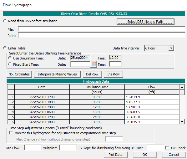
The two upstream boundary conditions used a flow hydrograph that was selected by highlighting the Boundary Condition cell and pressing the Flow Hydrograph button. The window where the Flow Hydrograph data is entered is shown in the figure below. The user may select to read hydrograph data from a DSS file or manually enter the flow data in the table provided. For this example the flow hydrograph was manually entered for RS -933.33 of the Ohio River while a DSS file was read in for the upstream BC for the Upper Mississippi.

For River Station -933.33 of the Ohio River, the Data Time Interval was set to six hours and the radio button Use Simulation Time was selected. The Use Simulation Time option starts the hydrograph at the beginning of the simulation time window, which is discussed in an upcoming section. The hydrograph was then manually entered after first clicking the Enter Table radio button.

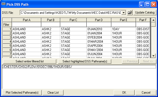
The flow hydrograph associated with the upper reach of the Mississippi River (RS 110.4) differed from the Ohio River upstream boundary condition in that it pulled its flow information from a DSS file. A DSS file was connected to the RS by pressing the button Select DSS file and Path. When this button was pressed a DSS file and pathname selection screen appeared as shown in the figure below. The desired DSS file was found and selected by using the browser button at the top. Once the DSS file was selected, a list of all of the DSS pathnames within that file was displayed in the table. The pathname filters were used to reduce the number of pathnames shown in the table. When the desired DSS pathname was found the window was closed and the filename and pathname will be recorded in the Flow Hydrograph Window.

Downstream Boundary Condition

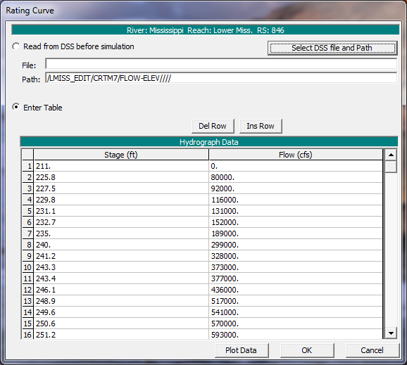
The boundary condition selected for RS 846 of the Lower Mississippi was a rating curve. Again, the corresponding cell for that particular river station was highlighted and then the Rating Curve button was selected. A window appeared as seen in the figure below where the radio button Enter Table was clicked and the stage and flow values were manually entered.

Internal Boundary Conditions

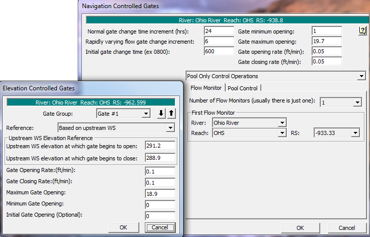
Internal boundary conditions were entered for the gates of the two inline structures and to represent un-modeled tributaries. The inline structure at RS -938.8 of the Ohio River utilized "Navigation Dams" BC, while the inline structure at RS -962.599 used the "Elev Controlled Gates" BC. The data for these two BC were entered as seen in the figure below. For more information on entering data for Elev Controlled Gates or Navigation Dams see Chapter 8 and 16 of the User's Manual.

Lateral inflow hydrographs were added throughout the river reaches as a means of representing flow from an un-modeled tributary. This is often done when there is un-modeled tributary flow that has a noticeable impact on the modeled system but the impact of the modeled floodwave on the tributary is not considered to be within the scope of the model's objective. Therefore, the effects of the flow are captured without having to model unnecessary parts of the system. For all five of the lateral inflow hydrographs used in this example, the hydrograph was read in from DSS. This was done in the same manner as was the flow hydrographs for the upstream BC (explained above).

Initial Conditions

Initial conditions consist of flow information at each of the cross sections, as well as elevations for any storage areas defined in the system. Data for initial conditions is established by selecting the Initial Conditions tab on the Unsteady Flow Data Editor. After selecting the tab, the figure below will be displayed.

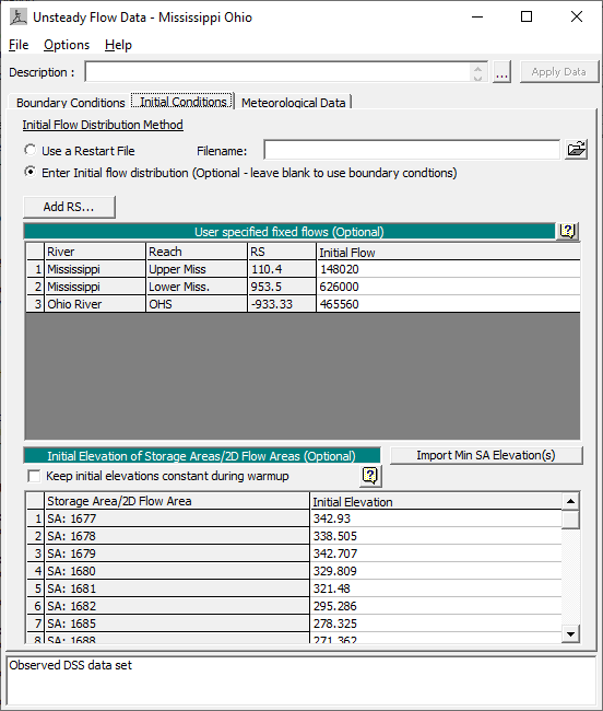
As seen in the figure above, the Enter Initial flow distribution radio button was selected and initial flows were entered at the upstream river station of each of the three reaches. The initial water surface elevation of all twenty-seven storage areas was set as well. The data was then saved (File -> Save Unsteady Flow Data As) in the Unsteady Flow Data Editor and the window was closed.

Unsteady Flow Analysis

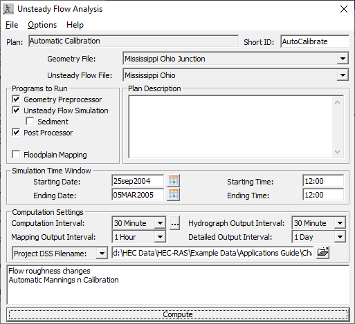
After the geometry and unsteady flow data have been completed an unsteady flow analysis may be initiated. Under the main program window Unsteady Flow Analysis was selected under the Run menu. This displayed the Unsteady Flow Analysis Window shown in the figure below. A plan was defined by selecting the Geometry File "Mississippi Ohio Junction" and the Unsteady Flow File "Mississippi Ohio." Under the File menu, Save Plan As was selected and the plan title was entered as "Automatic Calibration." After entering the title of the plan a short identifier was entered as "AutoCalibrate" and the plan was saved. The data was entered as seen in the figure below. For more information on the Simulation Time Window, Computation Settings, and Programs to Run refer to Unsteady Flow Application – Example 17.

Calibration of Manning's n Values

In an effort to ensure a higher level of model accuracy, the user can calibrate the model when reliable gage data is available. Often times the primary focus of calibration is the adjustment of Manning's n values. However, before the user begins adjusting any Manning's n values they should consider the following:

• If the model is predicting stages that have a large degree of variance from the historic events, the users should also evaluate the hydrologic data and the geometric data to ensure that it is correct. Things such as incorrect hydraulic structure coefficients or flow data can make a significant impact on the results.

• Manning's n values should initially be determined using a combination of site visits, aerial photography, topographic maps, experience, etc. The initial estimate for Manning's n values should be used as a baseline for reasonable values when calibrating. If the calibrated n values are drastically different from the initial values, the user should critically evaluate the model to find any possible errors or mistaken assumptions. Do not proceed with calibration using unreasonable or unrealistic Manning's n values.

Adding Observed (Measured) Data

As alluded to previously, in order to calibrate Manning's n values in HEC-RAS the user must have a reliable and accurate gage(s) within the system. In this example nine time-series DSS gages were used – three for each reach. Gages can be added from the Options menu of the Unsteady Flow Data Editor. Under Options the user can select three types of observed data from Observed (Measured) Data: Time Series in DSS, High Water Marks, or Rating Curves (Gages).

In this example the Time Series in DSS option was selected. Once selected, a window appeared titled "Set Locations and Paths for Observed Data in DSS" that allows the user to match a DSS file to a river location (see figure below). The river and river station were chosen from the three drop down menus at the top of the window: River, Reach, and River Sta. Once the correct location was set, the Add selected location to table was clicked and the location was added to the table below. Next, the DSS file was added from the DSS File option (middle of the window). When the DSS file was connected, the table below was automatically populated with the DSS file pathnames, which contained the observed values.

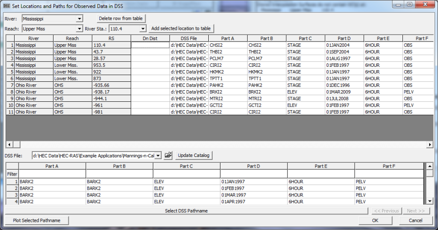
Finally, the appropriate DSS file and pathname was connected to each individual RS in the top table by highlighting the desired row and then selecting the corresponding gage data (pathname) from the bottom table. The information from the pathname selected in the bottom table should then be populated in the highlighted row in the top table. In this example, Part A, Part B, and Part C columns of the DSS file tell the user which gage location and data type (stage, flow, etc.) the user is selecting. It is important that the user is careful to match the DSS file with the correct location and required data type. However, matching column Part D, which has the time that the data begins, is not pertinent. It is not required that the date listed in Part D for the row that the user selected fall within the simulation time of the model. As long as the gage has collected data during the simulation time frame, HEC-RAS will automatically find the corresponding gage times. The pathname data can be visually inspected by clicking the Plot Selected Pathname button in the lower left hand corner of the window.

Calibration of Base Manning's n Values

Once all the Manning's n values have been entered for each cross section, the observed data has been entered, and the plan has been processed, the user can evaluate the output to determine if the base Manning's n values need to be adjusted to better match the observed conditions. In this example, some of the RS with gage data calculated stage values that were either consistently above or below the observed values. This indicated that all of the Manning's n values near that RS needed to be adjusted either up or down, depending on whether it over- or under-estimated the river stage.

The Manning's n values can be easily manipulated by opening Manning's n or k values (Horizontally varied) from the Tools menu of the Geometric Data Editor. The figure below will then appear and the desired River and Reach can be selected, as well as the region of the river (in this case All Regions was always selected).

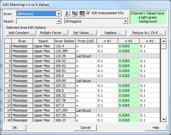
If it were the case that the stage values were consistently to low for RS 43.7 of the Upper Mississippi River, the channel (highlighted in green) and overbank Manning's n values near RS 43.7 could be selected and adjusted upward by a factor of 1.05 by clicking the Multiply Factor from the Selected Area Edit Options above the table. This would increase all of the highlighted Manning's n values by 5%. This change would increase the stage near and upstream of RS 43.7 when the plan was reprocessed. Alternatively, the Add Constant or Set Values could have been selected to change the Manning's n values.

Automatic Calibration of Manning's n

Manually calibrating base Manning's n values can often times be a tedious, challenging (especially if it is a complex system), or even impossible task. Occasionally, simulated flow hydrographs will overestimate at some portions of the hydrograph while underestimating at other portions at the same river station, making it impossible to calibrate the values at all locations, for all flow rates (low to high). This can be due to stream geometry variations during different times/seasons or could be due to variances in stream behavior during different flow rates. Both of these factors can be accounted for through the Options menu of the Unsteady Flow Analysis. However, for this example only the Flow Roughness Factors tool (seen in figure below) will be evaluated since the user is required to create flow roughness factors when using the automated calibration procedure. Note: The flow roughness factors can also be accessed from the Tools selection of the Geometric Data Editor's menu. However, accessing it from the Geometric Editor will relate the flow roughness factors to the geometry file and not the plan file. Although either set of flow roughness factors can be used for automated calibration, the user should beware of this distinction and use the option according.

Once the Flow Roughness Factor Editor was opened, the first thing that was done was to divide each river reach into segments that correspond to each gage. Typically, it is ideal to have the gage at the upstream portion of each river segment. For example, the gage at 43.7 of the Upper Mississippi had a corresponding river segment ranging from the upstream RS of 43.7 to the downstream RS 29.09 (immediately upstream of the next gage). This was done by selecting Mississippi, Upper Miss, 43.7, and 29.09 from the River, Reach, Upstream Riv Sta, and Downstream Riv Sta dropdown menus, respectively. As seen in the figure below, flow values were entered in the bottom table so that all possible flows were accounted for in the table. Next, a corresponding roughness factor was entered for each flow value. After the table was filled in, the Add button was selected and the other river segments were created in the same manner.

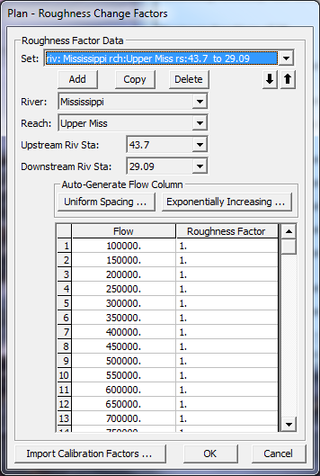
As mentioned earlier, the automated calibration procedure computes adjustments to existing flow roughness factors to follow observed stages. An initial set of flow roughness factors must already be set in the geometry or plan and the observed stages must already be in the unsteady flow data before implementing this calibration procedure. In this example, the initial flow vs. roughness factors are all being set to a value of 1.0 (no change to the base n values), since the automated calibration process will be computing flow vs roughness factors for us. After the initial set of flow versus roughness factors were set up for all of the reaches to be calibrated, the Automated Roughness Calibration tool was accessed from the Options menu of the Unsteady Flow Analysis Editor. The Unsteady Roughness Calibration Editor appears as in the figure below. There are four distinct regions within the editor: Calibration Parameters, Calibration Regions, Forcing Internal Observed Flows, and Forcing Internal Observed Stages. The last two are not thoroughly discussed in this example because they were not used. The user is encouraged to look to Chapter 16 of the User's Manual for more information on the Unsteady Roughness Calibration Editor.

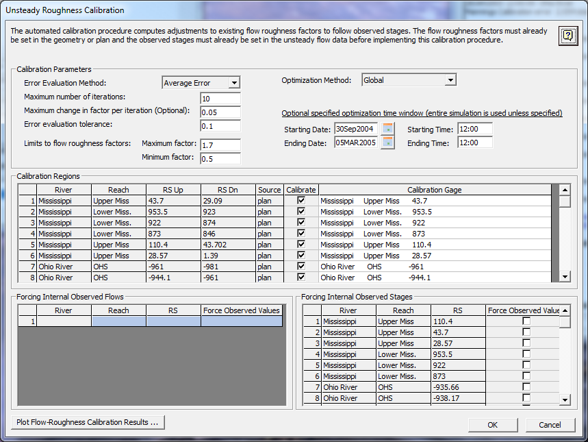
First, the fields within the Calibration Parameters region were entered. The Optimization Method was set to Global. The other possible selection from the dropdown was the sequential method. The sequential method can potentially lead to better results; however, it takes much longer to run because it goes through many more iterations. Computationally, the primary distinction between the two methods is that the global method calibrates all Manning's n values simultaneously, whereas the sequential method calibrates the upstream river stations first and then works its way down to the lower river stations. Also, for sequential method calibration, the bottom two regions – Forcing Internal Observed Flows and Forcing Internal Observed Stages – must be used; however, they are not used with the global method.

Next, the remaining fields within the Calibration Parameters were filled in. The Error Evaluation Method was set to Average Error for this example. The Maximum number of iterations and Maximum change in factor per iteration were set to 10 and 0.05, respectively. The iteration tolerance is the acceptable convergence error, which basically tells the program what amount of error the user is comfortable with and when to stop running. This value was set to 0.1 for this example. In layman's terms - for the entries of this example - these parameters tell the program that it has up to ten attempts to get an error under 0.1 while adjusting the factors by no more than 0.05 (5%) on any iteration and keeping its estimates within a range of 0.5 and 1.7. The limit placed on the amount changed per iteration is used to keep the program from overshooting the best answer, while the range ensures that the final answer isn't something unreasonable. An optional time window was also used for this example. The start date was five days after the simulation time and ended at the same time as the simulation (25 Sep 2004 – 05 Mar 2005). This function can be used if the user doesn't want to evaluate a certain portion of the flow hydrograph.

The Calibration Regions portion of the window was completed next. This area was already populated with the roughness factor river segments that were created earlier. Under the Calibration Gage column, a gage was paired with the river segment that it corresponded to by selecting the cell and then choosing the appropriate gage from a drop down menu that appeared. Lastly, each box under the Calibrate column heading was checked on.

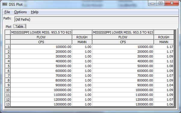
The OK button was clicked and the Unsteady Flow Analysis was run. After the model ran, the new calibrated Manning's n values can be found by reopening the Unsteady Roughness Calibration Editor and clicking the Plot Flow-Roughness Calibration Results button in the lower left hand corner of the window. A DSS plot will appear (see figure below) that displays pre- and post-calibration roughness factors. The first tab plots the data, while the second tab (as seen in the figure below) displays the results in a table. If the user is satisfied with the calibrated roughness factors, they can copy and paste them into the Flow Roughness Factor Editor so that the new values will be used in the next run.

Output Analysis

The best way to check the validity of the calibrated hydrograph and the impact of the adjustment in roughness factors is by comparing the pre- and post-calibrated stage and flow hydrographs.

Stage and Flow Hydrographs

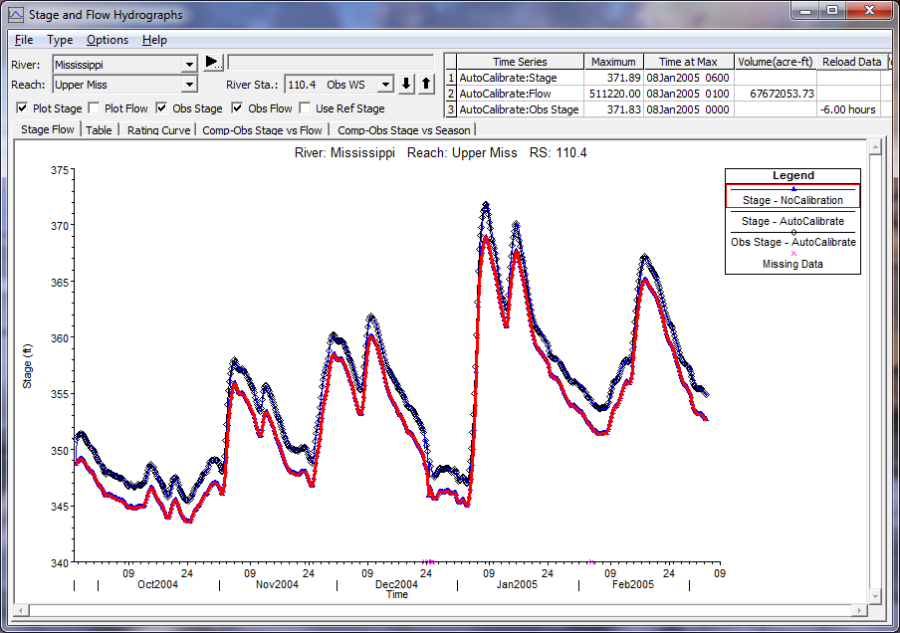
The stage and flow hydrographs can be opened by choosing Stage and Flow Hydrographs from the Run selection of the main menu bar. The observed stage (black line with diamonds), calibrated stage (blue line), and the originally calculated stage (red line) can be seen in . As seen in the figure, the calibrated hydrograph nearly perfectly matches the observed hydrograph, whereas the original, uncalibrated hydrograph is consistently underestimating the gage values.

Summary

This example demonstrated how to set up a gaged unsteady flow model that was calibrated with HEC-RAS's Automated Roughness Calibration feature. The user was first shown how to set up the geometric data, unsteady flow data, and the unsteady flow analysis. The primary focus however was demonstrating how to use the Flow Roughness Factors Editor and the Automated Roughness Calibration feature. Once the model was calibrated, the results were found in a DSS plot from the Automated Roughness Calibration Editor. The output was then analyzed by comparing the observed, calibrated, and originally simulated stage hydrographs. The importance of calibrating a model should be made clear from this example. What also should be conveyed is that the Automated Roughness Calibration feature makes calibration much quicker and simpler.