Multiple Culverts - Example 4

This example is designed to demonstrate the use of HEC-RAS to analyze the flow of water through multiple (non-identical) culverts. The program has the capability of analyzing flow through a single type of culvert, multiple identical types of culverts, and multiple non-identical types of culverts. A culvert type defines the characteristics of the culvert, which includes the shape, slope, roughness, chart, and scale number. For a given culvert type, the program can analyze up to 25 identical barrels. This example analyzed two culvert types, each with two identical barrels.

The entering of data and the analysis of these culverts was identical to the procedures used for the single culvert type as performed for Example 3. Additionally, the data used for Example 3 was modified for this example to include a second culvert type. Therefore, Example 4 is presented as a continuation of Example 3 and the modeler should review the data and the procedures as performed in Example 3 before reviewing Example 4.

The user is referred to Example 3 for the basic procedures of culvert analyses and to Chapter 6 of the Hydraulic Reference Manual for a detailed discussion on modeling culverts. To review the procedures performed for this example, from the main HEC-RAS window, select File and then Open Project. Go to the directory in which you have installed the HEC-RAS example data sets. From the "Applications Guide\Example 4 – Multiple Culverts" subdirectory, select the project labeled "Multiple Culverts - Example 4." This will open the project and activate the following files:

Plan: "Spring Creek Multiple Culverts"
Geometry: "Multiple Culvert Geometry"
Flow: "Multiple Culvert Flow Data"

Example 4 - Multiple Culverts.zip

Geometric Data

To perform the analysis, the geometric data was entered first. The geometric data consists of the river system schematic, the cross section geometry, placement of the cross sections, and the culvert information. Each of these geometric data components are described in the following sections.

River System Schematic

From the main program window, select Edit and then Geometric Data and the river system schematic of Spring Creek will appear as shown in the figure below. This river reach is defined by ten river stations, with river station 20.535 as the upstream cross section and river station 20.000 as the downstream cross section. The schematic is identical to the river reach as developed during Example 3.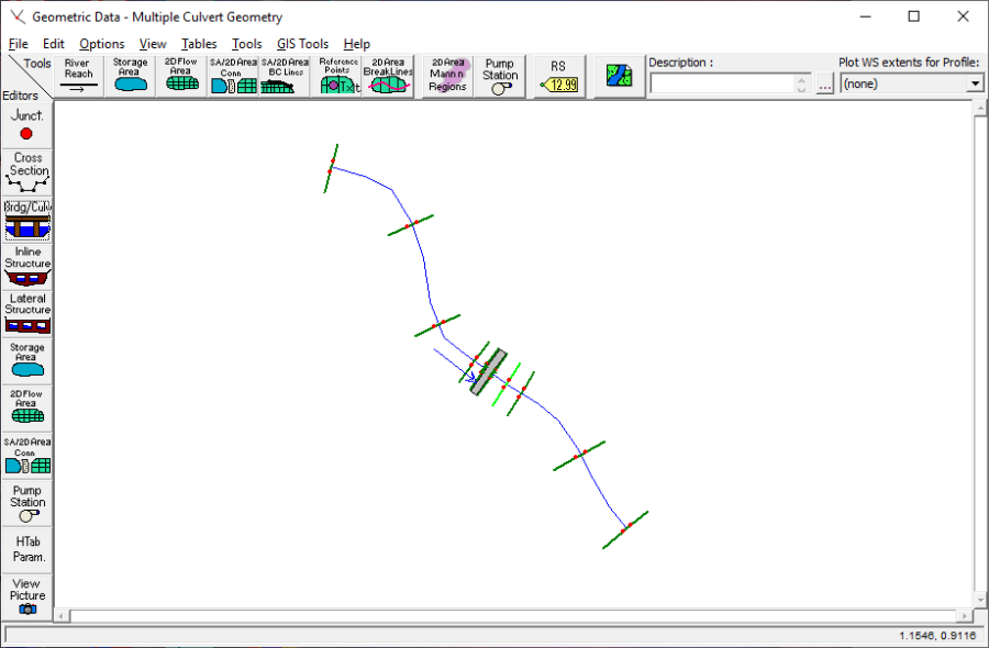 River System Schematic for Spring Creek

Cross Section Geometry

The geometry of the cross sections for this example are identical to the geometry of the cross sections for Example 3. The modeler should review Example 3 for the stationing, elevations, reach lengths, Manning's n values, main channel bank stations, and contraction and expansion coefficients determined for each cross section. (Note: The Manning's n values for the LOB and ROB at river stations 20.238 and 20.227 were reset to the original value of 0.1.) Finally, the ineffective flow areas for the cross sections in the vicinity of the culvert were adjusted after the additional culvert information was added.

Expansion and Contraction Reach Lengths

The placement of cross sections in reference to the culvert, define the expansion and contraction reach lengths. These reach lengths are crucial for the accurate prediction of the energy losses through the culvert. The determination of the reach lengths was discussed in detail during Example 3. During the analysis, it was observed that an additional cross section was required to be added to account for the expansion of the flow. This additional cross section was added as cross section number 20.208*, with the * indicating that the cross section was interpolated using the methods available by the program. After the analysis for this example, the expansion and contraction reach lengths were again evaluated and will be discussed near the end of this example.

Culvert Data

The culvert data consists of entering the deck/roadway data and the culvert geometric data. Each of these areas will be discussed as follows.

Deck/Roadway Data. The deck and roadway data editor is activated from the main program window by selecting Edit, Geometric Data, the Bridge/Culvert icon, and then the Deck/Roadway icon. This will display the Deck/Roadway Data Editor as shown in Example 3. The values for this current example were exactly the same as those entered for Example 3.

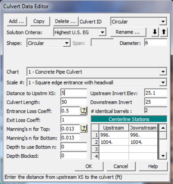
Culvert Geometric Data. To enter the culvert geometric data, from the Bridge/Culvert Data Editor select the Culvert icon. This will activate the Culvert Data Editor and display the data for culvert #1 as shown in the figure below. Culvert #1 is defined exactly as described for Example 3: a circular culvert of diameter 6 feet with two identical barrels and the other parameters as shown in the figure below. In the upper right corner of the editor, the Rename button was selected and the new name "Circular" was entered. This will help the modeler during the review of the output for this example.

The output analysis of Example 3 showed that during the flow of 600 cfs, the flow overtopped the roadway and created weir flow. For this current example, we will consider the possibility that the flow must not overtop the roadway and that the modeler desires to install additional culverts to alleviate this problem. Alternatively, to reduce the upstream water surface depth, the modeler has extensive options available such as increasing the diameter of the existing culverts or adding other identical barrels to the culvert. For this example, however, the option of installing additional culverts was pursued.

From the Culvert Data Editor (as shown in the figure above), the Add button in the upper left corner was selected. This cleared the entry fields and created a new input window as shown in the figure below. The identification name "Culvert #2" appeared in the Culvert ID field in the upper right corner of the editor. The Rename button, located immediately below the Culvert ID, was selected and a new name "Box" was entered. The additional fields of the Culvert Data Editor will be described as follows.

Solution Criteria - The user has the option to select to use the result for inlet control or outlet control as the final answer for the upstream energy grade line value. The default method is to use the highest of the two values, as was selected for this example.

Shape - The culvert shape is chosen from the eight available shapes: circular, box, elliptical, arch, pipe arch, semi-circle, low or high arch. For this second culvert, the culvert shape was selected as box. To select the shape, press the down arrow on the side of the shape field and highlight the desired shape.

Diameter, Rise, or Rise and Span - Depending on the shape of the culvert, the modeler must enter the inside dimensions of the culvert shape. For a box shape, the rise (vertical distance) and span (horizontal distance) must be entered. A value of 5 feet for the span and 3 feet for the rise were entered. (Note: For box culverts with chamfered corners, refer to the discussion in Chapter 6 of the Hydraulic Reference Manual.)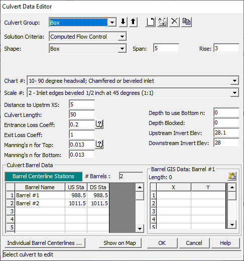 Box Culvert Data Editor

Chart # - Each culvert type and shape is defined by a Federal Highway Administration Chart Number. Depress the down arrow next to this field to select the appropriate chart number. Once a culvert shape has been selected, only the corresponding chart numbers available for that culvert shape will appear in the selections. Descriptions for the chart numbers appear in Chapter 6 on Table 6.5 of the Hydraulic Reference Manual. For this example, the culvert chart was selected as "10 - 90 degree headwall; Chamfered or beveled inlet edges."

Scale - This field is used to select the Federal Highway Administration scale that corresponds to the selected chart number and culvert shape. Only the scale numbers which are available for the selected chart number will appear for selection. Descriptions for the scale numbers appear in Chapter 6 on Table 6.5 of the Hydraulic Reference Manual. The scale for this example was "2 - Inlet edges beveled ½ in / ft at 45 degrees (1:1)."

Distance to Upstream XS - This is the distance from the inlet of the culvert to the upstream cross section (20.238). For this example, this was a distance of 5 feet. On the Deck/Roadway Data Editor, a measure of 10 feet was entered for the distance from the upstream side of the deck/roadway to the upstream cross section. Therefore, the culvert entrance is located midway between the upstream side of the roadway and cross section 20.238.

Length - This field is the measure of the culvert (in feet or meters) along the centerline of the barrel. The length of the culvert for this example is 50 feet.

The program will add this 50 feet to the 5 foot distance from cross section 20.238 (to the culvert entrance) and obtain 55 feet. The reach length from cross section 20.238 to 20.227 is 57 feet, which leaves 2 feet from the exit of the culvert to the downstream cross section.

Entrance Loss Coefficient - The value of the entrance loss coefficient will be multiplied by the velocity head at the inside upstream end of the culvert to obtain the energy loss as the flow enters the culvert. Typical values for the entrance loss coefficient can be obtained from Tables 6.3 and 6.4 in the Hydraulic Reference Manual. The entrance loss coefficient for the concrete box culvert was set at 0.2.

Exit Loss Coefficient - To determine the amount of energy lost by the water as it exits the culvert, the exit loss coefficient will be multiplied by the difference of the velocity heads from just inside the culvert at the downstream end to the cross section located immediately downstream from the culvert exit. In general, for a sudden expansion, the exit loss coefficient should be set equal to 1. However, this value may range from 0.3 to 1.0. For this example, the exit loss coefficient was set to be equal to 1.0.

Manning's n for Top - This field is used to enter the Manning's n value of the top and sides of the culvert lining and is used to determine the friction losses through the culvert barrel. Suggested n values for culvert linings are available in many textbooks and also may be obtained from Table 6.1 in the Hydraulic Reference Manual. Roughness coefficients should be adjusted according to individual judgment of the culvert condition. For this example, a Manning's n value of 0.013 was used for the concrete culverts.

Manning's n Value for Bottom – This field is used to enter the Manning's n value of the bottom of the culvert. For most culverts, this field will be the same as the Manning's n value for the top. However, if the culvert has a natural bottom, or something has been placed in the bottom for fish passage, the n value may vary.

Depth to use Bottom n – This field is used to enter a depth inside of the culvert that the bottom n value is applied to. If the bottom and top n value are the same, a value of zero should be entered.

Depth Blocked – This field is used to fill in a portion of the culvert. The user enters a depth, and everything below that depth is blocked out.

Upstream and Downstream Invert Elevation - These two fields are used to enter the elevations of the inverts. For a particular culvert type, all of the identical barrels will have the same upstream invert elevation and downstream invert elevation. For this example, the upstream invert was set at an elevation of 28.1 feet and the downstream invert was 28.0 feet.

Barrel Centerline Stations - This table is used to enter the stationing (X-coordinates) of the centerlines of the culvert barrels. The upstream centerlines are based upon the X-coordinates of the upstream cross section (20.238) and the downstream centerlines are based upon the X-coordinates of the downstream cross section (20.227). This example employs two culvert barrels, with the centerlines of the barrels occurring at stations 988.5 and 1011.5 feet, as measured on both cross sections. For this example, the X-coordinate geometry of both cross section 20.238 and cross section 20.227 are referenced from the same left station starting point. Therefore, the upstream and downstream centerline stations are the same value and this will align the culvert in the correct configuration as being parallel to the channel. The modeler must be cautious to ensure that the centerline stationing of the culvert ends align the culvert in the correct position.

# Barrels - This field will automatically display the number of barrels entered by the user (determined by the number of centerline stations entered). Up to 25 identical barrels can be entered for each culvert type, and this box culvert consisted of 2 identical barrels.
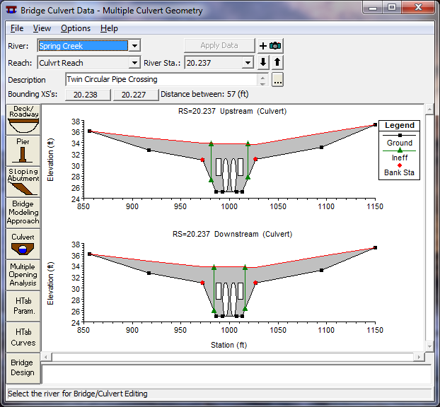
This completed the necessary geometric data for the culverts. The OK button was selected and the final configuration of the culverts is as shown in the figure below. (Note: The ineffective flow areas will be adjusted subsequently.) The modeler should now close the editor and save the data.

Box and Circular Culverts at River Station 20.237

Ineffective Flow Areas

Since additional culverts were added at cross section 20.237, the ineffective flow areas at river stations 20.238 and 20.227 were adjusted for the new geometry. From the Geometric Data Editor, the Cross Section icon and river station 20.238 were selected. Select Options and then Ineffective Flow Areas. This activated the Ineffective Flow Area Data Editor as shown in the figure below.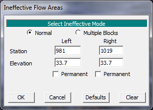
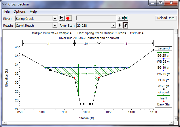
Ineffective Flow Area at River Station 20.238

The stationing of the ineffective flow areas at cross section 20.238 can be determined by using a 1:1 relationship to the distance of cross section 20.238 from the culvert entrance. For this example, cross section 20.238 is located 5 feet upstream from the culvert entrance. Therefore, the left ineffective flow station was set at 5 feet to the left of the left edge of the culvert openings. The left edge of the culvert opening is at station 986. This places the left ineffective flow station at station 986 - 5 = 981 feet. Similarly, the right ineffective flow station was set to be 5 feet to the right of the right edge of the culvert opening. This equates to station 1014 + 5 = 1019. The elevation of the ineffective flow areas will remain as originally set for Example 3, at an elevation of 33.7 feet.

The ineffective flow areas at cross section 20.227 are determined in a similar manner as used for cross section 20.238; however, cross section 20.227 is placed at a distance of 2 feet downstream of the culvert exit. Therefore, the ineffective flow stationing at cross section 20.227 is 984 and 1016 for the left and right stations, respectively. The elevations for the ineffective flow areas at cross section 20.227 were set at 33.6, a value slightly lower than the lowest downstream high cord elevation.

This completed the required geometric data and the information was saved as the geometry file "Multiple Culvert Geometry."

Steady Flow Data

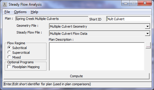
To perform the steady flow analysis, from the main program window Run and then Steady Flow Analysis were selected. This activated the window as shown in the figure below. The geometry file "Multiple Culvert Geometry," the steady flow file "Multiple Culvert Flow Data," and a subcritical flow regime were selected. A Plan title of "Spring Creek Multiple Culverts" was entered, as well as a Short ID of "Mult Culvert" and then the COMPUTE button was selected to perform the steady flow analysis.

Steady Flow Analysis

Output Analysis

To review the output, the modeler has various options and procedures. For this analysis, evaluations will be performed for: the expansion and contraction reach lengths, the channel contraction and expansion coefficients, and the water surface profiles.

Expansion and Contraction Reach Lengths

Initially, during Example 3, the expansion and contraction reach lengths were determined using table values obtained from the USACE research document \[HEC-1995\]. These reach length values were then compared to the actual distances of the expansion reach length (from cross section 20.227 to cross section 20.189) and the contraction reach length (from cross section 20.251 to cross section 20.238). It was then determined that the contraction reach length was adequate for the analysis; however, the estimated expansion reach length was less than the distance from cross section 20.227 to cross section 20.189. Therefore, an additional cross section, 20.208*, was interpolated and included as the location where the flow would fully expand. After the analysis for Example 3, the expansion and contraction reach lengths were computed using regression equations and compared to the predetermined values. For this current example, the regression equations will again be used to evaluate the expansion and contraction reach lengths.

Expansion Reach Length. Cross section 20.208* was the interpolated section that was assumed to be at the location where the flow became fully expanded. To evaluate the location of this cross section, the relationship shown below was used. It is applicable when the width of the floodplain and the discharge is less than those of the regression data. The equation is:

$\begin{array}{l}\displaystyle ER = \frac{L_e}{L_{obs}}=0.421+0.485\left( \frac{F_{20.227}}{F_{20.208^*}} \right)+0.000018Q\end{array}$

where

$\begin{array}{l}ER\end{array}$ = expansion ratio
$\begin{array}{l}L_e\end{array}$ = expansion reach length, ft
$\begin{array}{l}L_{obs}\end{array}$ = average length of side obstruction, ft
$\begin{array}{l}F_{20.227}\end{array}$ = main channel Froude number at the cross section immediately downstream of the culvert (cross section 20.227 for this example)
$\begin{array}{l}F_{20.208^*}\end{array}$ = main channel Froude number at the cross section of fully expanded flow (cross section 20.208* for this example)
$\begin{array}{l}Q\end{array}$ = total discharge, ft³/s

(Note: The subscripts used and all subsequent equations reflect the river station numbering for this example.) From the analysis, the Froude numbers at cross sections 20.227 and 20.208* for the flow of 600 cfs are 0.18 and 0.14, respectively. Substituting these values into this equation yields an expansion ratio of 1.06. The standard error for this equation is 0.26, which yields a range of the ER from 0.80 to 1.32 to define the 68% confidence band. For this current example, the average length of obstruction is determined to be approximately equal to 60 feet. With this length of obstruction, the expansion reach length is:

$\begin{array}{l}\displaystyle L_e = \left( ER \right) \left( L_{obs} \right) = \left( 1.06 \right) \left(60 \right) = 64 \ ft\end{array}$

This is the median value of the range from 50 to 80 feet (using ER = 0.80 and 1.32, respectively). The actual distance from cross section 20.227 to cross section 20.208* was set at 100 feet, which is only slightly greater than the maximum value of the range as determined from the equation above. Therefore, the existing reach length was not adjusted. Also, since the regression equation was based on studies conducted for low flow through bridges and since the flow for this example is less than the flow rates used to develop the equation, the expansion reach length was not adjusted from the existing value. Finally, the resulting expansion ratio should not exceed 4:1 nor should it be less than 0.5:1.

Contraction Reach Length. Cross section 20.251 is located where the flow lines are parallel to the main channel. To evaluate this location, the equation shown below will be utilized. This equation is used when the floodplain scale and dischargers are significantly different than those used in the regression analysis and is:

$\begin{array}{l}\displaystyle CR = 1.4-0.333 \left( \frac{F_{20.227}}{F_{20.208^*}} \right) + 1.86 \left( \frac{Q_{ob}}{Q} \right)^2 -0.19 \left( \frac{n_{ob}}{n_c} \right)^{0.5}\end{array}$

where

$\begin{array}{l}CR\end{array}$ = contraction ratio
$\begin{array}{l}L_c\end{array}$ = contraction reach length
$\begin{array}{l}Q_{ob}\end{array}$ = discharge conveyed by the two overbanks at cross section 20.251, cfs
$\begin{array}{l}Q\end{array}$ = total discharge, cfs
$\begin{array}{l}n_{ob}\end{array}$ = Manning's n value for the overbanks at section 20.251
$\begin{array}{l}n_c\end{array}$ = Manning's n value for the main channel at cross section 20.251

From the analysis of the 600 cfs profile, the flow in the two overbanks at cross section 20.251 was 34.54 cfs and the Manning's n values for the overbanks and main channel at cross section 20.251 are 0.10 and 0.04, respectively. Substituting these values into the equation above yielded a contraction ratio of 0.68. The standard error for this equation is 0.19, which yields a CR range from 0.49 to 0.87 to define the 68% confidence band. This range is less than the range obtained from Table B-2 of 0.8 - 1.5. Using the contraction ratio of 0.8 and an average obstruction length of 60 feet, the contraction reach length is:

$\begin{array}{l}\displaystyle L_c = \left( CR \right) \left( L_{obs} \right) = \left( 0.8 \right) \left( 60 \right) = 48 \ ft\end{array}$

Channel Expansion and Contraction Coefficients

The coefficients of expansion (Ce) and contraction (Cc) for flow in the cross sections are used to determine the energy losses associated with the changes in channel geometry. Initially, in the vicinity of the culvert, the coefficients were set at 0.5 and 0.3 for the expansion and contraction, respectively. Each of these values will be reviewed.

Expansion Coefficient. The expansion coefficient can be obtained from the equation below:

$\begin{array}{l}\displaystyle C_e = -0.09+0.570 \left( \frac{D_{ob}}{D_c} \right) + 0.075 \left( \frac{F_{20.227}}{F_{20.208^*}} \right)\end{array}$

where

$\begin{array}{l}C_e\end{array}$ = coefficient of expansion
$\begin{array}{l}D_{ob}\end{array}$ = hydraulic depth (flow area divided by the top width) for the overbank at cross section 20.208*
$\begin{array}{l}D_c\end{array}$ = hydraulic depth for the main channel at cross section 20.208*

From the analysis of the 600 cfs profile, the hydraulic depths for the overbanks and the main channel at river station 20.208* are 0.58 and 5.66 feet, respectively. Substitution of the values into this equation yields an expansion coefficient of 0.07. This is the median value and the range of ± 0.2 defines the 95% confidence band for the equation above. For this example, a value of 0.5 was used. The value of the expansion coefficient is generally larger than the value used for the contraction coefficient so the value of 0.5 will remain as the selected value. The modeler can perform a sensitivity of this coefficient by changing this coefficient and performing subsequent analyses. For this example, the change in velocity head from cross section 20.227 to 20.208* was only 0.06 feet. Since this value is small, a change in the expansion coefficient will only reflect a minor change in the resulting water surface elevation.

Contraction Coefficient. From the research document \[HEC-1995\], the contraction coefficient is obtained by first determining the relationship:

$\begin{array}{l}\displaystyle b/B=28/145 \approx 0.20\end{array}$

where

$\begin{array}{l}b\end{array}$ = culvert opening width, ft (m)
$\begin{array}{l}B\end{array}$ = total floodplain width, ft (m)

From Table B-3 in Appendix B of the Hydraulic Reference Manual, the recommended contraction coefficient range is 0.3 - 0.5. The value selected for this example was the minimum value of 0.3.

Water Surface Profiles

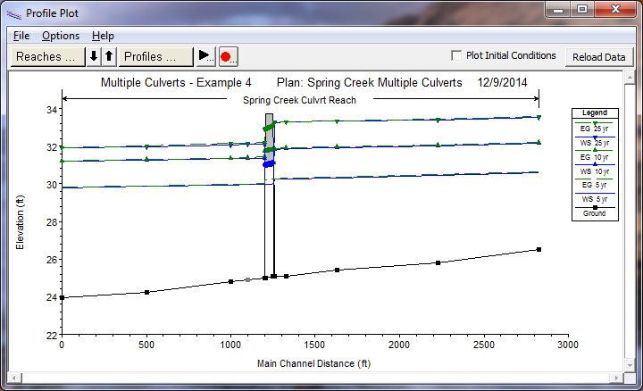
From the main program window, select View and then Water Surface Profiles. This will result in the display as shown in the figure below. In the figure, the water surface profiles are shown for all three flows. As can be seen in the figure, the water surface for the first flow (250 cfs) was able to travel through the culverts without submerging the inlet or outlet. For the second and third flow profiles, it can be seen that the culvert entrance was submerged but that weir flow did not occur for either flow.

Water Surface Profiles For Spring Creek

To analyze this further, the modeler can view the profile output table to determine the depths of flow at the upstream side of the culverts. From the main program window, select View, Profile Table, Std. Tables, and then Culvert Only. This will display the table as shown in the figure below.

Culvert Only Profile Table

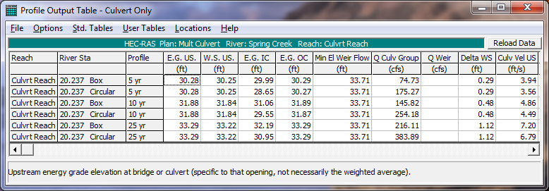
In the this figure, the first two rows are for the flow through the box and circular culverts for the flow of 250 cfs. Then the second set of rows are for the flow of 400 cfs, and finally the last two rows are for the flow of 600 cfs. For both the box and the circular culverts, the upstream inside top elevation was set at 31.1 feet. By comparing this value to the upstream water surface elevation (W. S. US.), it is determined that both of the culverts were submerged at the entrance for the second and third flow profiles because the upstream water surface elevations were 31.83 and 33.22 feet, respectively.

Additional analysis of the table reveals that outlet control was the type of flow occurring through the culvert for all 3 flow profiles, because the outlet energy grade line was greater than the inlet control energy grade line. The flow through each culvert, for each flow profile, is shown in the column with the heading "Culv Q." For example, for the first flow profile (250 cfs), there was 74.73 cfs flowing through the box culverts (37.36 cfs through each barrel) and 175.27 cfs flowing through the circular culverts (87.64 cfs through each barrel). This totals 74.73 + 175.27 = 250 cfs and accounts for the total flow rate for the first flow profile. Finally, there are no values in the weir flow column of the table, which signifies that weir flow did not occur for these flow rates. This was an initial goal to develop a culvert system that produced no weir flow. The modeler can now determine the available freeboard on the upstream side of the roadway embankment and adjust the sizes and shapes of the culvert as deemed necessary.

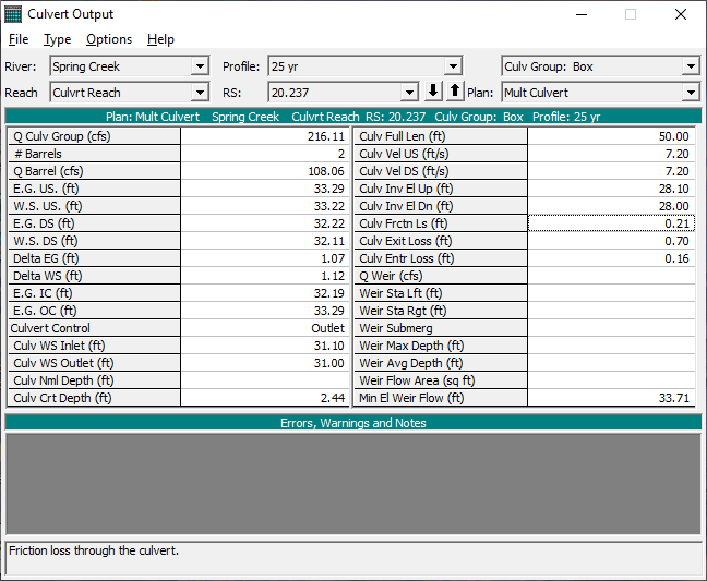
For a more detailed analysis of each culvert, select View, Cross Section Table, Type, and then Culvert. Toggle to profile 3 (600 cfs) and select the "Box" as the Culvert ID. This will display the table as shown in the figure below. This table displays additional information for the selected culvert and flow profile such as the length of the culvert flowing full and the energy losses. The modeler can compare these losses with values obtained for other entrance and exit loss coefficients. Finally, as displayed on the previous table, it can be seen that there is no weir flow occurring at this river station. The modeler can then toggle to the circular culvert at this river station by selecting the Culvert ID field. If additional culverts were located at other river stations, the data for these culverts can be viewed by selecting the appropriate river station.

Culvert Type Cross Section Table

Finally, the location of the ineffective flow areas will be reviewed. From the main program window, select View and then Cross Sections. Toggle to river station 20.238 and this will display the cross section as shown in the figure below. In the figure, it can be seen that the water surface elevations did not exceed the elevations set for the ineffective flow areas. Additionally, toggle to river station 20.227 and it can be seen that the water surface elevation is lower than the elevations set for the ineffective flow areas at this cross section. Since weir flow did not occur, the ineffective flow areas set for cross sections 20.238 and 20.227 should reasonably reflect the actual flow conditions.

Cross Section 20.238 of Spring Creek

Summary

This example demonstrated the use of HEC-RAS to analyze a river reach that contained a multiple culvert opening. The multiple culverts consisted of two culvert types (circular and box), each with two identical barrels. After the flow analysis was completed, the expansion and contraction reach lengths were evaluated and the ineffective flow areas were reviewed. Finally, the various output features (flow profiles, cross section type tables, and profile tables) were displayed to show the features available for a review of the output.