Download PDF
Download page Single Bridge (WSPRO) - Example 13.
Single Bridge (WSPRO) - Example 13
The field data for this example were obtained from the United States Geological Survey (USGS) Hydrologic Atlas No. HA-591. This atlas is one part of a series developed to provide data to support hydraulic modeling of flow at highway crossings in complex hydrologic and geographic settings. The bridge, cross section geometry, and high water flow data were used to evaluate two flood flows. The first flood had a peak discharge of 25000 cfs and occurred on December 7, 1971, constituting a recurrence interval of 50 years. The second event had a peak discharge of 31500 cfs and occurred on March 25, 1973, with a recurrence interval greater than 100 years. It should be noted that modelers typically do not have access to high water marks and actual field flow measurements at bridges during the peak events. However, for this example, since the observed peak water surface elevations were available, they were compared to the output from HEC-RAS.
For this analysis, the water surface profiles were determined by using the WSPRO \[FHWA, 1990\] routine, which is an available low flow bridge hydraulics method in the HEC-RAS program. This example will focus upon the entering of data and review of the output for a bridge analysis using the WSPRO method. The user should be familiar with entering bridge data, as performed for Example 2. The user is referred to Chapter 5 of the *Hydraulic Reference Manual* and to Chapter 6 of the *User's Manual* for additional discussion concerning bridge analyses.
To review the data files for this example, from the main HEC-RAS window, select *File* and then *Open Project{*}. Go to the directory in which you have installed the HEC-RAS example data sets. From the "Applications Guide\Example 13 – Single Bridge (WSPRO)" subdirectory, select the project labeled "Bogue Chitto, MS - Example 13." This will open the project and activate the following files:
Plan:"WSPRO Bridge Analysis"
Geometry:"Bridge Crossing near Johnston Station"
Flow: "50 and 100 year flows"
 Example 13 - Singler Bridge (WSPRO).zip
Geometric Data
The geometric data for this example consists of the river system schematic, cross section data, cross section placement, bridge geometric data, ineffective flow areas, and the bridge modeling approach. Each of these items are discussed below.
River System Schematic
To view the river system schematic, from the main program window select Edit and then Geometric Data. This will activate the Geometric Data Editor and the screen will display the schematic, as shown in the below. For this example, the river system is composed of one river and only one reach. The river is labeled "Bogue Chitto" and the river reach is "Johnston Sta." The river system was defined initially with 11 cross sections beginning at river mile 50.00 as the downstream cross section and river mile 56.97 as the upstream cross section. The initial cross section data were obtained from the USGS Atlas, and cross sections were interpolated along the river reach to provide additional cross section data.
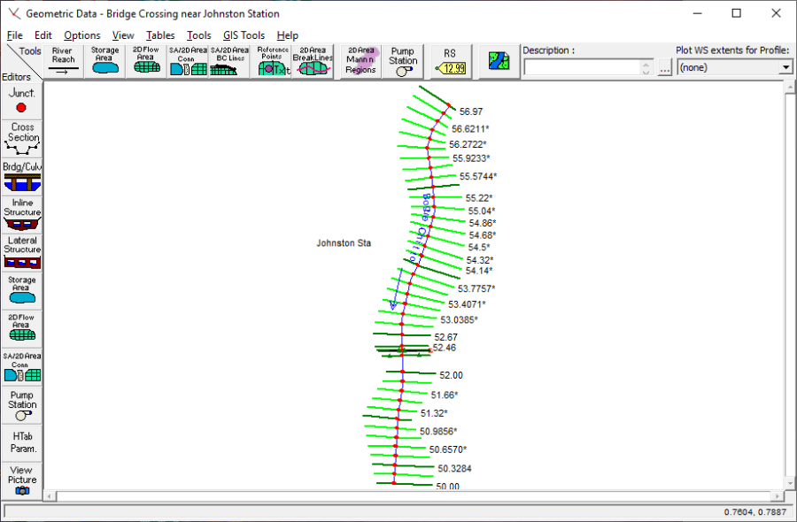
The editing commands of Add Points to a Reach and Move Object were used to curve the river system schematic. This was performed for aesthetic purposes only, and does not effect the hydraulic computations.
Cross Section Geometric Data
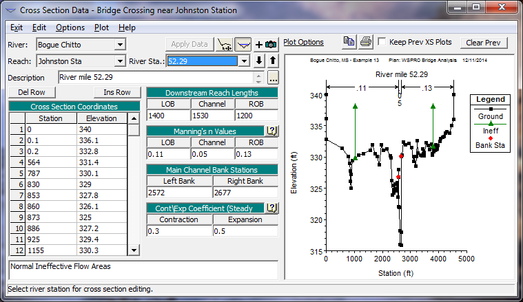
To enter the cross section data, the Cross Section icon on the left side of the Geometric Data Editor was selected. This activated the Cross Section Data Editor, as shown in the top figure below. Then, Add a new cross section was selected under the Options menu to create each new cross section. For each cross section, the geometric data consisted of the: description, X-Y coordinates, reach lengths, Manning's n values, main channel bank stations, and contraction and expansion coefficients. (Note: The ineffective flow areas will be discussed in a subsequent section.)
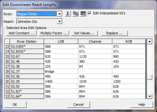
Manning's n values, and main channel bank stations were obtained from the field data displayed on the USGS atlas. A summary table of the reach lengths, Manning's n values, or contraction and expansion coefficients for the cross sections can be seen by selecting the relevant listing under the Tables menu on the Geometric Data Editor. The summary table of the reach lengths for the cross sections is shown in the bottom, figure below.
Cross Section Placement
The reach lengths, as shown in the figure above, determine the placement of the cross sections. The placement of the cross sections relative to the location of the bridge is crucial for accurate prediction of expansion and contraction losses. The bridge routine utilizes four cross sections to determine the energy losses through the bridge. (Additionally the program will interpret two cross sections inside of the bridge by superimposing the bridge data onto both the immediate downstream and upstream cross sections from the bridge.) The following is a brief summary for the initial estimation of the placement of the four cross sections. The modeler should review the discussion in Chapter 6 of the User's Manual and Chapter 5 of the Hydraulic Reference Manual for further detail.
First Cross Section. Ideally, the first cross section should be located sufficiently downstream from the bridge so that the flow is not affected by the structure (i.e., the flow has fully expanded). This distance (the expansion reach length) should generally be determined by field investigation during high flows and will vary depending on the degree of constriction, the shape of the constriction, the magnitude of the flow, and the velocity of the flow. In order to provide better guidance to determine the location of the fully expanded cross section, a study was performed by the Hydrologic Engineering Center \[HEC-1995\]. This study focused on determining the expansion reach length, the contraction reach length, and the expansion and contraction energy loss coefficients. The results of the study are summarized in Appendix B of the Hydraulic Reference Manual. To determine an initial estimate of the expansion reach length, the following information was required:
| b=450 \ ft \\ B = 5000 \ ft \\ b/B = 0.1 \\ S = (25.7 \ ft )/ (36790 \ ft) \cdot (5280 \ ft/mi) = 3.7 \ ft/mi \\ n_{ob}/n_{ch} = (0.13)/(0.05) = 2.6 \\ L_{obs} = 1770 \ ft |
where:
b = bridge opening width
B = total floodplain width
S = slope
n_{ob = Manning's n value for the overbank
n_{chManning's n value for the main channel
L_{obs = average length of the side obstructions
With the above information, an initial estimate of the expansion reach length (Le) was obtained by using the table values in Appendix B of the Hydraulic Reference Manual. From Table B.1, an average value of the expansion ratio (ER) was 1.2. Using this value, the expansion reach length is:
| L_e = \left( ER \right) \left( L_{obs} \right) = (1.2)(1770 \ ft) = 2120 \ ft |
From the reach lengths table (above), the distance from cross section 52.36 to 52.00 is 1956 feet (= 426 + 1530). Therefore, cross section 52.00 was initially considered as the cross section of fully expanded flow. Since cross section 52.29 is in the zone of flow expansion, ineffective flow areas were placed in the overbank areas. This will be discussed further during the determination of the ineffective flow areas. After the steady flow analysis was performed, the expansion reach length was evaluated using regression equations that are presented in the HEC study \[HEC-1995\]. The equations require flow parameters at the initially chosen location and cannot be evaluated until after the steady flow analysis is performed. These procedures will be described near the end of this example.
Second Cross Section. The second cross section used by the program to analyze the energy losses through the bridge is located a short distance downstream of the structure. This section should be very close to the bridge and reflect the effective flow area on the downstream side of the bridge. For this example, a roadway embankment sloped gradually from the roadway decking on both sides of the roadway. Cross section 52.36 was located at the toe of the roadway embankment and was used to represent the effective flow area on the downstream side of the bridge opening. The program will superimpose the bridge geometry onto this cross section to develop a cross section inside the bridge at the downstream end.
Third Cross Section. The third cross section is located a short distance upstream from the bridge and should reflect the length required for the abrupt acceleration and contraction of the flow that occurs in the immediate area of the opening. As for the previous cross section, this cross section should also exhibit the effective flow areas on the upstream side of the bridge. For this example, cross section 52.38 was located at the toe of the roadway embankment on the upstream side of the bridge. Similar to the previous cross section, the program will superimpose the bridge geometry onto this cross section to develop a cross section inside the bridge at the upstream end.
Fourth Cross Section. The fourth cross section is located upstream from the bridge where the flow lines are parallel and the cross section exhibits fully effective flow. To determine an initial estimate of the contraction reach length \left( L_c \right), a value of the contraction ratio (CR) was obtained as 0.8 from Table B.2, Appendix B of the Hydraulic Reference Manual. This yields a contraction reach length of:
| L_c = \left( CR \right) \left(L_{obs} \right) = (0.8)(1770 \ ft) = 1400 \ ft |
From the reach lengths table (see recent figure above), the distance from cross section 52.46 to 52.38 is 380 feet. For this example, cross section 52.46 was initially used as the section where the flow lines were parallel. After the steady flow analysis, the location of this cross section was evaluated using the procedures as outlined in the recent HEC study [HEC-1995]. This evaluation will be presented in the discussion near the end of this example.
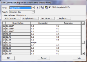
Additionally, the HEC study [HEC-1995] provided guidance to determine the expansion and contraction coefficients. The contraction and expansion coefficients are used by the program to determine the transition energy losses between two adjacent cross sections. From the data provided by the recent HEC study \[HEC-1995\], gradual transition contraction and expansion coefficients are 0.1 and 0.3, and typical bridge contraction and expansion coefficients are 0.3 and 0.5, respectively. For situations near bridges where abrupt changes are occurring, the coefficients may take larger values of 0.5 and 0.8 for contractions and expansions, respectively. A listing of the selected values for the river reach can be viewed by selecting Tables and then Coefficients from the Geometric Data Editor. This table is shown in the figure below and displays the values selected for the river cross sections. Typical gradual transition values were selected for stations away from the bridge. However, near the bridge section, the coefficients were increased to 0.3 and 0.5 to represent greater energy losses. For additional discussion concerning contraction and expansion coefficients at bridges, refer to Chapter 5 of the Hydraulic Reference Manual. After the steady flow analysis, the selection of the coefficients were evaluated and will be discussed near the end of this example.
This completed the input for the cross section geometric data. Next, the bridge geometry data was entered as outlined in the proceeding section.
Bridge Geometry Data
To perform the hydraulic analysis, the bridge geometry was entered next. This section provides a brief summary of the input for the bridge geometry including the bridge deck/roadway, sloping abutments, and bridge piers.
Bridge Deck and Roadway Geometry. From the Geometric Data Editor, select the Bridge/Culvert icon. To create the bridge cross sections, the river was selected as "Bogue Chitto," the reach was "Johnston Sta," and then Options and Add a Bridge and/or Culvert were selected. The bridge river station was then entered as 52.37. Next, the data for the bridge deck were entered. The Deck/Roadway icon was selected and the Deck/Roadway Data Editor appeared as shown in figure below.
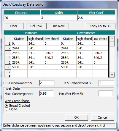
The first input at the top of the editor is the distance from the upstream side of the bridge deck to the cross section immediately upstream from the bridge (cross section 52.38). This distance was determined to be 26 feet from the USGS atlas. In the next field, the bridge deck width of 31 feet was entered. This is a total distance of 31 + 26 = 57 feet. From the reach lengths table (see Cross Section Placement figure), the distance from cross section 52.38 to 52.36 is 84 feet. This leaves 84 - 57 = 27 feet from the downstream side of the bridge deck to cross-section 52.36. Finally, at the top of the Deck/Roadway Data Editor, a weir flow coefficient of 2.6 was selected for the analysis.
The central section of the Deck/Roadway Editor is comprised of columns for input of the station, high cord elevation, and low cord elevation for both the upstream and downstream sides of the bridge deck. The data were entered from left to right in cross section stationing and the area between the high and low cord comprised the bridge structure. The stationing of the upstream side of the deck was based on the stationing of the cross section located immediately upstream. Likewise, the stationing of the downstream side of the deck was based on the stationing of the cross section placed immediately downstream. If both the upstream and downstream data are identical, the user needs only to input the upstream data and then select Copy Up to Down to enter the downstream data.
As a final note, the low cord elevations that are concurrent with the ground elevation were entered as a value lower than the ground elevation. The program will automatically clip off and remove the deck/roadway area below the ground. For example, at station 0, a low cord elevation of 0 feet was entered. However, the actual ground elevation at this point is approximately 340 feet. Therefore, the program will automatically remove the area of the roadway below the ground. Additionally, the last station was entered as a value of 5000 feet. This stationing ensured that the roadway and decking extended into the limits of the cross section geometry. As described previously, the program will clip off the area beyond the limits of the cross section geometry.
Below the deck station and elevation data, there are two fields to enter the upstream and downstream embankment side slopes. These values are used by the WSPRO bridge analysis method and for graphical representation on the profile plot. For this example, values of 2.0 (horizontal to 1 vertical) were entered for both the US Embankment SS and DS Embankment SS, as measured from the USGS Atlas.
At the bottom of the Deck\Roadway Data Editor, there are three additional fields for data entry. The first is the Max Allowable Submergence. This input is a ratio of downstream water surface to upstream energy, as measured above the minimum weir elevation. When the ratio is exceeded, the program will no longer consider the bridge deck to act as a weir and will switch the computation mode to the energy (standard step) method. For this example, the default value of 0.95 (95 %) was selected.
The second field at the bottom of the editor is the Min Weir Flow Elevation. This is the elevation that determines when weir flow will start to occur over the bridge. If this field is left blank (as for this example), the program will default to use the lowest high cord value on the upstream side of the bridge. Finally, the last field at the bottom of the editor is the selection of the weir flow submergence method. This method will determine the reduction of the weir flow coefficient due to submergence. For this example, a broad crested weir flow submergence method was selected. Upon entering all of the above data, the OK button was selected to exit the Deck/Roadway Data Editor.
Bridge Pier Geometry. To enter the pier data, the Pier icon was selected from the Bridge/Culvert Data Editor. This resulted in the display shown in the figure below. The modeler should not include the piers as part of the ground or bridge deck/roadway because pier-loss equations use the separate bridge pier data during the computations.
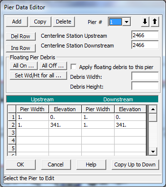
The program will establish the first pier as pier number 1. As shown in the figure above, the upstream and downstream stations were entered for the centerline of the first pier. The upstream and downstream stations were based on the geometry of the cross sections located immediately upstream (cross section 52.38) and immediately downstream (cross section 52.36) of the bridge. The user needs to be cautious placing the pier centerline stations because the X-coordinates for the upstream and downstream cross section stationing may be different. This is to ensure that the piers "line up" to form the correct geometry. For this example, the 17 piers are placed 24 feet on center, with centerline stationing from 2466 to 2850. The piers are 1 foot wide for their entire height. The starting elevation is set below the ground, and the ending elevation is inside the bridge decking. With these elevations, the program will "clip off" the excess pier heights. After entering the data, the OK button was selected.
Sloping Abutments. The next icon on the left side of the Bridge/Culvert Data Editor is Sloping Abutment. This icon was selected to enter the abutment data, and is shown in the figure below for the first (left) abutment. The user can view the data for the second (right) abutment by selecting the down arrow on the Sloping Abutment Data Editor in the HEC-RAS program. After the data were entered, the OK button was selected to exit the editor and the schematic of the bridge/deck, piers, and abutments was displayed as is shown in the figure proceeding the figure below. (Note: The figure in the text displays the ineffective flow areas that will be added in the next section.)
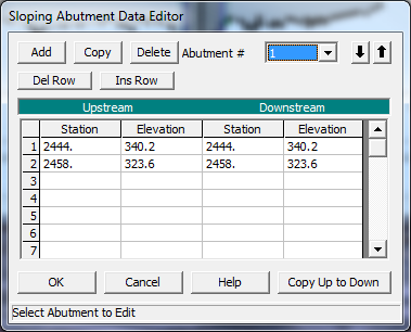
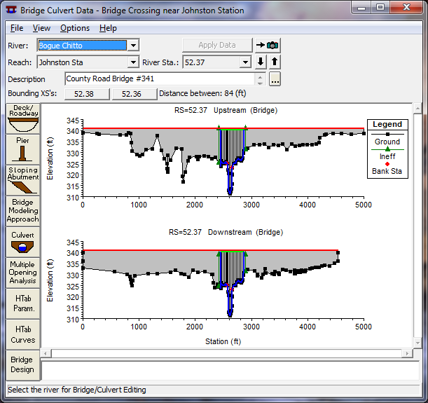
The cross sections shown in the figure below are developed by superimposing the bridge data on the cross sections immediately upstream (52.38) and immediately downstream (52.36) of the bridge. The top cross section in the figure below reflects the geometry immediately inside the bridge on the upstream side and the bottom cross section reflects the geometry immediately inside the bridge on the downstream side.
While viewing the bridge, the modeler can select to view just the upstream, just the downstream, or both of the cross section views. This is performed by selecting View and then the required option. Additionally, from the View menu, the user should select Highlight Weir, Opening Lid and Ground as well as Highlight Piers. These options enable the modeler to view what the program will consider as the weir length, bridge opening, and pier locations. Any errors in the data will appear as inconsistent images with these options. Also, the zoom-in option will allow the user to examine data details. Finally, the Apply Data button was selected to accept the data. (Note: To save the data to the hard disk, the user must select Save Geometry Data under the File menu on the Geometric Data Editor).
Ineffective Flow Areas
As a final step for the bridge geometry, any ineffective flow areas that existed due to the bridge (or any other obstruction) were entered. Ineffective flow is used to define an area of the cross section in which the water will accumulate but is not being actively conveyed. At a bridge, ineffective flow areas normally occur just upstream and downstream of the road embankment, away from the bridge opening.
For this example, ineffective flow areas were included on both the upstream cross section (52.38) and the downstream cross section (52.36), as well as on cross section 52.29 (the cross section in the expansion reach). To determine an initial estimate for the stationing of the ineffective flow areas on either side of the bridge, a 1:1 ratio of the distance from the bridge to the cross section was used. For this example, cross section 52.38 is located 26 feet upstream of the bridge. Therefore, the left and right ineffective flow areas were set to start at 26 feet to the left and right of the bridge opening. The left side of the bridge opening is at station 2444, which leads to a left ineffective station of 2444 - 26 = 2418. The right side of the bridge opening is at station 2864, which leads to a right ineffective flow station of 2864 + 26 = 2890. Similarly, cross section 52.36 is located 27 feet downstream from the bridge and the ineffective flow areas at this cross section were set at 27 feet to the left and right of the bridge opening, at stations of 2417 (= 2444 - 27) and 2891 (= 2864 + 27), respectively.
The initial elevation of the ineffective flow areas for the upstream cross section was chosen as 340.8, a value slightly lower than the lowest high cord elevation (341.0). This ineffective flow elevation was chosen so that when the water surface becomes greater than this ineffective elevation, the flow would most likely be weir flow and would be considered as effective flow.
At the downstream cross section, the elevation of the ineffective flow area was set to be 339.0, slightly lower than the low cord elevation (340.2). This elevation was chosen so that when weir flow occurs over the bridge, the water level downstream may be lower than the low cord, but yet it will contribute to the active flow area.
The ineffective flow areas were entered by first selecting the Cross Section icon from the Geometric Data Editor. Then, Options and Ineffective Flow Areas were chosen for cross section 52.38 and then for cross section 52.36. The ineffective stations and elevations as previously determined were entered, as shown in the figure below for cross section 52.38.
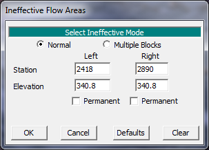
Since the "Normal" type of ineffective flow was chosen, these entries imply that all the water to the left of the left station and to the right of the right station will be considered as ineffective flow until the water level exceeds the elevation of 340.8 feet.
Cross section 52.29 is in the area of expanding flow and therefore only a portion of the cross sectional flow will be effective. A "Normal" type of ineffective flow areas were set at stations 1030 and 3800, both at an elevation of 338. These stations were determined by taking into account the distance of cross section 52.29 from the bridge (426 feet), as compared to the total distance of the expansion reach length (1956 feet). With these distances, cross section 52.29 is located approximately 25% (= 426 / 1956 * 100%) down the expansion reach length. As the flow exits the bridge opening, it will initially expand at a greater rate than it will farther downstream. An initial estimate of the degree of expansion was assumed to be approximately 60% at cross section 52.29. Therefore, 60% of the left overbank width was subtracted from the left main channel bank station to determine the left ineffective flow station. Similarly, 60% of the right overbank width was added to the right main channel bank station to determine the right ineffective flow station. The elevation of 338 was chosen to be greater than the water surface elevations.
The OK button was selected and then Apply Data was chosen to accept the data. The ineffective flow areas then appeared as triangles, as shown in the previous figure above for the bridge cross-sections. Additionally, the ineffective flow areas will appear on the cross sections plots. Finally, a note will appear in the box at the bottom of the Cross Section Data Editor that states an ineffective flow exists for each cross section that this option was selected for, as shown in the second to top figure on this page. The ineffective flow areas could have been entered previously along with the discussion of the cross section data (X-Y coordinates, reach lengths, etc.). However, it is often easier to enter the bridge data first and then the ineffective flow data to easily determine where the ineffective flow stations should be located. After the steady flow analysis was performed, the ineffective flow areas were evaluated to determine if they were placed appropriately. This will be discussed near the end of this example.
Bridge Modeling Approach
The bridge routines in HEC-RAS allow the modeler to analyze the bridge flows by using different methods with the same geometry. The different methods are: low flow, high flow, and combination flow. Low flow occurs when the water flows only through the bridge opening and is considered as open channel flow (i.e., the water surface does not exceed the highest point of the low cord of the bridge). High flow occurs when the water surface encounters the highest point of the low cord of the bridge. Finally, combination flow occurs when both low flow or pressure flow occur simultaneously with flow over the bridge. The modeler needs to select appropriate methods for both the low flow and for the high flow methods. For the combination flow, the program will use the methods selected for both of the flows.
From the Geometric Data Editor, select the Bridge/Culvert icon and then the Bridge Modeling Approach button. This will activate the Bridge Modeling Approach Editor as shown in the figure below. For this example, there is only 1 bridge opening located at this river station and therefore the bridge number was 1. The modeler is referred to Chapter 6 of the User's Manual and Chapter 5 of the Hydraulic Reference Manual for additional discussion on the bridge modeling approach editor.
Low Flow Methods. The modeler needs to select which low flow methods the program should compute and which method the program should use. The modeler can select to have the program compute particular methods or all of the methods. Then, the modeler needs to select which method the program will use as a final solution. Alternatively, the modeler can select the computation of several or all of the methods, and then have the program use the method with the greatest energy loss for the final solution.
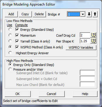
For this example, all four low flow methods were selected to be computed. For the momentum method, a drag coefficient Cd = 2.00 was entered for the square nose piers. For the Yarnell method, a value of K = 1.25 was entered. Finally, the WSPRO method was selected to be used for the solution. The modeler is referred to Example 2 - Beaver Creek for an example application that further discusses the low flow methods of energy, momentum, and Yarnell.
For the WSPRO method, the user is required to enter additional data. This was performed by selecting the WSPRO Variables button from the Bridge Modeling Approach editor. This activated the WSPRO Data Editor, as shown in the figure below. Most of the data entered on this editor is used to determine the "Coefficient of Discharge" for the WSPRO method. The following discussion outlines the WSPRO data that was entered for this analysis. The user is referred to Chapter 6 of the User's Manual and to Chapter 5 of the Hydraulic Reference Manual for a more detailed discussion of WSPRO method.
At the top of the editor, as shown in the figure below, the value of 341 feet was entered for the left and right elevations of the top of the embankments. The elevations for the toe of the abutments were entered as 323.6 and 330.5, for the left and right abutments, respectively. Next, the abutment type was selecting as type 3: sloping abutments and sloping embankments. The average slope of the abutments was entered as 1 (horizontal to 1 vertical) and the top width of the embankment was entered as 31 feet. All of these values were obtained from the USGS Atlas.
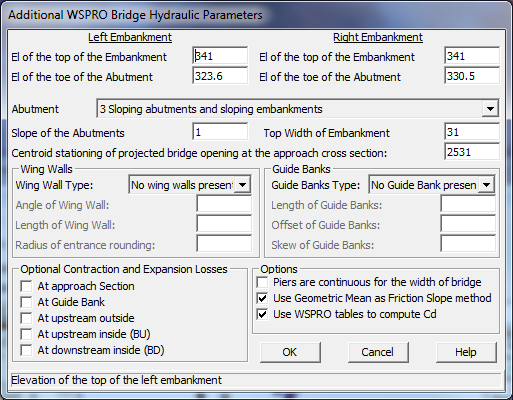
The centroid stationing of projected bridge opening at the approach cross section was entered as a value of 2531 feet. To obtain this value, the bridge opening width is projected onto the approach cross section (52.46). This projected width is situated onto the approach section such that the main channel is in the same relative position to the bridge opening width on the approach section as at the bride opening. The width of the projecting bridge opening should embrace the flow, which could pass through the actual bridge opening without contraction. Then, the centroid of the bridge opening width on the approach section was then determined to be at a stationing of 2531.
The bottom portion of the editor is divided into four sections. The first section is to describe the Wing Walls on the abutments. For this example, there were no wing walls present. If wing walls were present, the user can select either "Angular" or "Rounded," by depressing the down arrow adjacent to this field. Then, the appropriate data would be entered for the angle, length and radius fields, pertaining to the type of wing wall selected.
The second section is to describe the Guide Banks. For this example, there were no guide banks. If guide banks were present, the options are "Straight" or "Elliptical" to describe the type and then the user would enter the appropriate dimensions of length, offset, and skew.
The third section at the bottom of the editor is Optional Contraction and Expansion Losses. The WSPRO method includes friction losses throughout the bridge region for the calculations. However, the only contraction or expansion loss that is included is an expansion loss from the exit section (cross section 52.29) to the cross section immediately downstream from the bridge (52.36). The user can include additional losses at the approach section (52.46), at the guide banks, at the upstream outside contracted section (52.38), at the inside bridge upstream section (52.37 BU), and at the inside bridge downstream section (52.37 BD). For this example, there were no additional energy losses selected.
The final section of the editor is used to select options for the piers and friction slope method. If the piers are continuous, then the user should select Piers are continuous for the width of the bridge. This selection will determine a weighting factor in the determination of the "Coefficient of Q" discharge factor. Finally, the WSPRO method traditionally utilizes the geometric mean equation to determine the representative friction slope between two cross sections. If the Use Geometric Mean as Friction Slope Method is selected, then the program will use this method. If it is not selected, then the program will use the friction slope averaging method that has been selected by the user. (This is selected in the Steady Flow Analysis window by choosing Options, Friction Slope Methods, and then the appropriate choice. The default method is Average Conveyance. The user is referred to Chapter 7 of the User's Manual and to Chapter 2 of the Hydraulic Reference Manual for more information on friction slope methods.)
This completed the entry of the data for the WSPRO method as the low flow method. The OK button at the bottom of the editor was selected to exit the editor. Next, the high flow method was selected on the Bridge Modeling Approach Editor.
High Flow Methods. High flows occur when the water surface elevation upstream of the bridge is greater than the highest point on the low cord of the upstream side of the bridge. Referring to the seond most recent figure above, the two alternatives for the program to compute the water surface elevations during the high flows are: Energy Only (Standard Step) or Pressure and/or Weir Flow. The Energy Only (Standard Step) method regards the flow as open channel flow and considers the bridge as an obstruction to the flow. The Pressure Flow computations are divided into two scenarios. The first is when only the upstream side of the bridge deck is in contact with the water and the second is when the bridge constriction is flowing completely full. The program will begin to calculate either type of pressure flow when the computed low flow energy grade line is greater than the highest point of the upstream low cord. Weir Flow occurs when the upstream energy grade line elevation (as a default setting) exceeds the lowest point of the upstream high cord.
For this example, the high flow method was selected as energy. From the data on the USGS Atlas, the observed water surface elevations did not encounter the bridge deck, so therefore a high flow method of analysis was not anticipated. The user is referred to "Example 2 - Beaver Creek" for a bridge analysis that applied a high flow method.
At this point, all of the bridge data have been entered. The OK button was selected to close the Bridge Modeling Approach Editor and the Apply Data button was depressed on the Bridge/Culvert Data Editor before it was closed. Then, the geometry data was saved as the file "Bridge Crossing near Johnston Station" by selecting File and then Save Geometry Data As from the Geometric Data Editor.
As a final geometric component, a picture of the bridge has been included as a separate file. The red square on the river system schematic indicates that a picture has been added for that cross section. This picture was scanned from the USGS Atlas and saved as the file "chit.bmp." To view this picture, the user can select the View Picture icon from the left side of the Geometric Data Editor. When river station 52.37 is selected, the picture should appear. The user is referred to Chapter 6 of the User's Manual for a discussion on adding and viewing pictures to the river system schematic.
Steady Flow Data
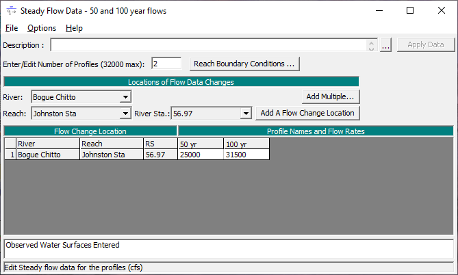
From the main program window, select Edit and then Steady Flow Data. This will display the Steady Flow Data Editor shown in the figure below (top). For this analysis on the reach of Bogue Chitto, two profiles were selected to be computed. The flow data were entered for river station 56.97 (the upstream cross section) and the flow values were 25000, and 31500 cfs. These flows will be considered continuous throughout the reach so no flow change locations were used. Additionally, the default profiles names of "PF#1 and "PF#2" were changed to "50 yr" and "100 yr," respectively. This was performed by selecting Edit Profile Names from the Options menu, and then typing in the new title.
Next, the boundary conditions were entered by selecting the Reach Boundary Conditions button. This resulted in the display shown in the figure below (bottom). For this example, a subcritical analysis was performed. Therefore, a downstream boundary condition was required for each flow value. The type of boundary conditions were known water surface elevations, therefore, Set boundary for one profile at a time was selected. With this selection, the table in the central portion of the editor expanded to show two rows, one for each of the two profiles. Then, the mouse arrow was placed over the downstream field for profile one and the box was selected (highlighted). The Known W.S. button was chosen and the data entry box appeared that requested the water surface elevation for the first profile. A value of 325.7 feet was entered, and the procedure was repeated for profile two, with a known water surface of 326.0 feet. These values were obtained from the USGS Atlas. The OK button was selected to exit the boundary conditions editor.
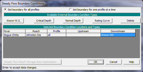
For the purposes of the analysis, if the downstream boundary conditions are not known, then the modeler should use an estimated boundary condition. However, this may introduce errors in the region of this estimated value. Therefore, the modeler needs to have an adequate number of cross sections downstream from the main area of interest so that the boundary conditions do not effect the area of interest. Multiple runs should be performed to observe the effect of changing the boundary conditions on the output of the main area of interest. For a detailed explanation of the types of boundary conditions, refer to Chapter 7 of the User's Manual and Chapter 3 of the Hydraulic Reference Manual.
A final optional component of the steady flow data was to enter the observed water surface elevation data from the USGS Atlas. This was performed by selecting Options and then Observed WS ... from the Steady Flow Data Editor. This activated the Observed Water Surface Data Editor, as shown in the figure below. The River was selected as "Bogue Chitto" and the Reach was "Johnston Sta." The observed values were entered for each of the two profiles, adjacent to the river stations that observed data was available for, as shown in the figure below. The OK button was then selected to exit the editor.
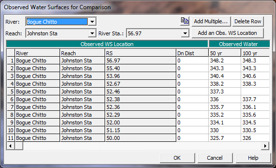
This completed the entry for the steady flow data. The Apply Data button was selected on the Steady Flow Data Editor and the flow data was then saved as "50 and 100 year flows."
Steady Flow Analysis
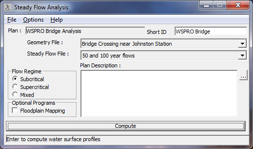
From the main program window, select Run and then Steady Flow Analysis. This will activate the Steady Flow Analysis Window as shown in the figure below. First, the geometry file and steady flow file that were previously developed should appeared in the selection boxes on the right side of the window. Then, for this simulation, a subcritical flow analysis was selected. Additionally, from the Steady Flow Analysis window, Options and then Critical Depth Output Option was selected. An "x" was placed beside the option for Critical Always Calculated. This may require additional computation time during program execution, but then the user can view the critical depth line during the review of the output for the cross sections. Select Options and then ensure that there is a check mark "" in front of Check data before execution. This will cause the program to check all of the input data to ensure that all pertinent information was entered. Next, a Short ID was entered as "wspro plan" and then the options were saved as a plan entitled "WSPRO Bridge Analysis." Finally, COMPUTE was selected at the bottom of the window.
Review of Output
After the program has completed the analysis, the last line should read "Finished Steady Flow Simulation." Click the Close button at the bottom of the window to close it. This review of the output will include discussions on the water surface profiles, profile summary tables, and detailed output tables.
Water Surface Profiles
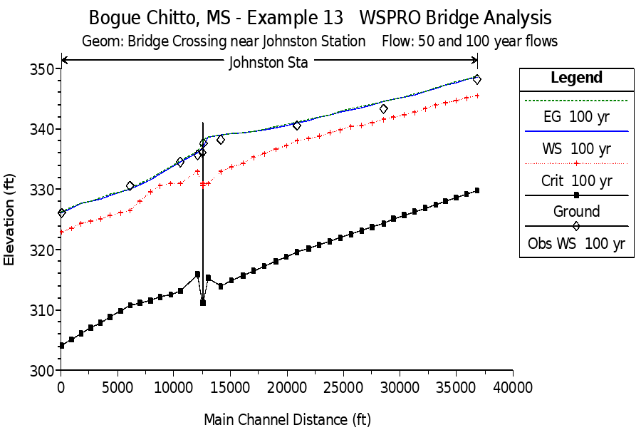
From the main program window, select View and then Water Surface Profiles. This will activate the water surface profile plot as shown in the figure below. In this figure, only the second profile was selected to be displayed, for clarity. This was accomplished by selecting Options, Profiles, and then profile 2. Additionally, the variables of Water Surface, Energy Grade Line, Critical Depth, and Observed Water Surface were selected to be displayed, by selecting Options and then Variables. The user can select additional profiles, variables, and the zoom feature under the Options menu when viewing the profile plot in the program.
The figure below displays a solid line for the water surface profile and a for the observed data, as shown in the legend. The water surface agrees well with the observed data. Additionally, it can be seen that the profile occurred in the subcritical flow regime. This ensures that for the low flow analysis, Class A low flow (subcritical flow) was occurring through the bridge. (This also occurred for the first profile.) To further review the output, the profile tables will be discussed next.
Profile Tables
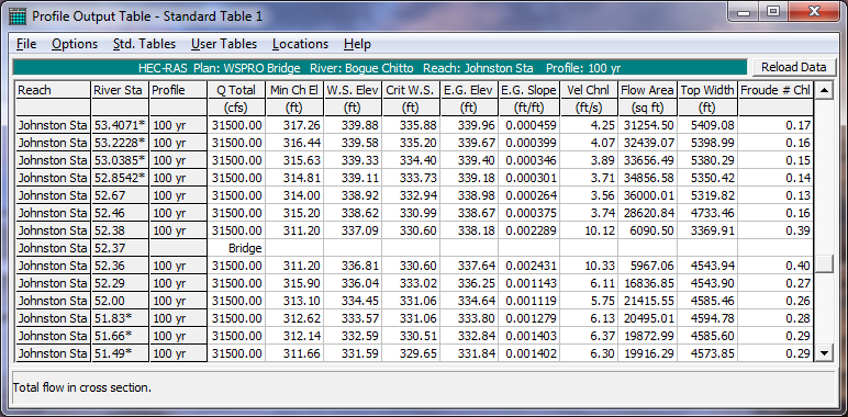
The profile tables are used to display the data for all of the river stations simultaneously. One type of profile table is the Standard Table 1 (below). This table can be activated by selecting from the main program window View, Profile Summary Table, and then Std. Tables, and Standard Table 1. This table displays the water surface elevation and energy grade line elevation (among other variables) for all the cross sections, and can be used to compare the calculated values to the observed water surface elevations. By selecting Options and Define Table, the additional column heading of "Obs WS" can be inserted prior to the "W.S. Elev." column. With these values displayed on the table, the user can easily compare the observed to the calculated values.
Another type of profile table is the Bridge Only table. This table is activated from the Std. Tables menu and is shown in the figure below, displaying the results for both profiles. The first row is for the first profile and the second row is for the second profile. The results in the table show the calculated values of the energy grade line at the cross section immediately upstream from the bridge (EG US) are 336.86 and 338.18 feet for the first and second profiles, respectively. The column heading Min El Prs shows a value of 340.20, which is the highest elevation of the low cord on the upstream side. If the energy grade line value had exceeded this elevation, then pressure flow would have been calculated. The Min Top Rd column shows the minimum elevation of the high cord on the upstream side. If the energy grade line had exceeded this value, then weir flow would have been calculated. Since the energy grade line for either profile did not exceed the low cord elevation, pressure flow, nor weir flow developed. This is also apparent since there are no values in the pressure only water surface (Prs O WS) or the weir flow (Q Weir) columns. The user is referred to "Example 2 - Beaver Creek" for an example where pressure and weir flow occurred.

To determine the method that was used for the final energy grade line value at the bridge, the Bridge Comparison table was activated from the Std. Tables menu, and is shown in the figure below. The two rows display the results for each of the two flow profiles, in ascending order. The river station in the second column is set at 52.37 (the only bridge location for this reach). The sixth through ninth columns show the results of the low flow methods that were chosen to be computed : Energy, Momentum, Yarnell and WSPRO methods, respectively. The values of the energy grade line that the program used is shown in the third column. As shown in Column five, the program used the result from the WSPRO method, as had been selected in the Bridge Modeling Approach Editor. Finally, the fourth column shows the water surface elevation that coincides with the energy elevation used by the program. (Note: There were no results in the last two columns for the high flow methods since only low flow occurred through the bridge opening.)
The results of the WSPRO method were only slightly greater than the results of the energy method. Both the momentum and Yarnell methods returned valid results since the water surface did not encounter the low cord of the deck. The user can adjust the input parameters of the WSPRO method to determine the significance of the values on the output, such as slope of the abutments and the inclusion of wing walls or guide banks.

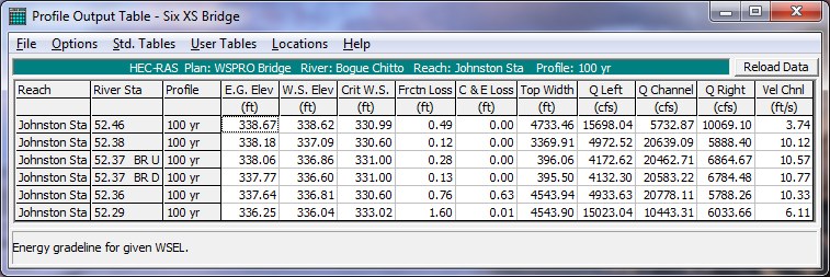
The final profile table that will be discussed is the Six XS Bridge table, which is also selected from the Std. Tables menu. This table is shown in the figure below, for profile 2. This table is specifically designed to show the data for the six cross sections that are used in the hydraulic computations through the bridge. The water surface and energy grade line values are shown in the first two columns of data, and are used to determine the water surface profile through the bridge. The C&E Loss column of the table shows the contraction or expansion losses. As shown in the figure, the only river station (within the six bridge cross sections) that had an expansion or contraction loss was river station 52.36 (to river station 52.29). This is because the WSPRO method, by default, only includes an expansion loss between the exit section and the cross section immediately downstream from the bridge. The user can include additional contraction/expansion losses by selecting the losses on the WSPRO Data Editor. For this example, no additional energy losses were selected, so no additional contraction or expansion losses appeared on the table.
Detailed Output Tables
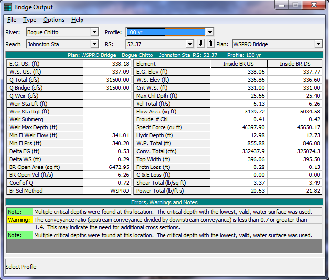
In addition to the profile tables, the user can view detailed output tables, which provide information at each specific cross-sections. A type of detailed output table that displays results for the bridge is shown in the figure below. This table was activated from the main program window by selecting View, Detailed Output Table, then Type and Bridge. The River and Reach were selected as "Bogue Chitto" and "Johnston Sta.", and the river station was 52.37 (the only river station that had a bridge). The Profile was selected as "2" and the Opening was "Bridge #1" (the only opening at this cross section). The table shows data for the cross sections inside the bridge, as well as the cross section just upstream from the bridge. As the user selects the different table fields, the description for the variables will appear at the bottom of the table. At the bottom of the left side of the table, the field Br Sel Mthd shows that the "WSPRO" results were used for the bride analysis. Additionally, the Coef of Q field shows that the WSPRO coefficient of Q value was calculated as 0.72 for the second profile.
At this time, the user can select to view the data for the first profile as well as viewing the cross section tables for the cross sections. This completed the review of the output for the cross section tables. Next, the locations of the cross sections in relation to the bridge were evaluated, by using the information presented in the various tables that were previously discussed.
Evaluation of Cross Section Locations
As stated previously, the locations of the cross sections and the values selected for the expansion and contraction coefficients in the vicinity of the bridge are crucial for accurate prediction of the energy losses through the bridge structure. For this example, the locations of the cross sections and the energy loss coefficients were evaluated for the second profile. The following analysis is based on data that were developed for low flow events occurring through bridges and the modeler should use caution when applying the procedure for other than low flow situations. Each of the reach length and coefficient evaluation procedures are discussed in the following sections.
Expansion Reach Length
The expansion reach length, Le, is defined as the distance from the cross section placed immediately downstream of the bridge to the cross section where the flow is assumed to have fully expanded. For this example, this distance is from cross section 52.36 to cross-section 52.00. Initially, the expansion reach length was estimated using the table values presented in Appendix B of the Hydraulic Reference Manual. After the analysis, the modeler can evaluate the initial estimate of the expansion reach length. For the analysis, it is recommended to use the regression results from the Army Corps of Engineers study [HEC-1995], which are summarized in the same Appendix B. The results of the study suggest the use of the equation below to evaluate the expansion reach length. This equation is valid when the modeling situation is similar to the data used in the regression analysis. (In the document, alternative expressions are presented for other situations.) The equation is:
| L_e = ER \left( \={L_{obs}} \right) = -298+257 \left( \frac{F_{52.36}}{F_{52.00}} \right) + 0.918 \={L_{obs}} + 0.00479Q |
where:
L_e
= expansion reach length, ft
ER = expansion ratio
F_{52.36} = main channel Froude number at the cross section immediately downstream of the bridge (cross section 52.36 for this example)
F_{52.00} = main channel Froude number at the cross section of fully expanded flow (initially cross section 52.00 for this example)
L_{obs}= = average length of obstruction caused by the two bridge approaches, ft
Q = total discharge, ft3/s
(Note: The subscripts used in this equation and all subsequent equations reflect the river station numbering for this example.)
From the field data, the average length of the obstruction is approximately 1770 feet and the total discharge, Q, is 31500 cfs for the high flow event. From the initial analysis, the value of the Froude number at cross-section 52.36 was 0.40 and at cross section 52.00 was 0.27 (as shown on Standard Table 1). Substituting the values into the equation above yielded that the expansion reach length, Le, was approximately 1874 feet. This equation has a standard error of 96 feet, which yields an expansion reach length range from 1778 to 1970 feet to define the 68% confidence band. The distance used for the expansion reach length (the distance from cross section 52.36 to cross section 52.00) was set to be 1956 feet in the main channel, which is approximately equal to the calculated distance of 1874 feet. Therefore, the expansion reach length was determined to be set appropriately.
If the reach lengths were not acceptable, then the modeler has the option to adjust the length so that it is within the calculated range. Then, after a new analysis, the new Froude numbers should be used to calculate a new expansion reach length. If the geometry is not changing rapidly in this region, then only 1 or 2 iterations should be necessary to obtain a constant expansion reach length value.
Contraction Reach Length
The contraction reach length, Lc, is defined as the distance from the cross section located immediately upstream of the bridge (52.38) to the cross section that is located where the flow lines are parallel and the cross section exhibits fully effective flow (52.46). To evaluate this reach length, the regression results (shown as the equation below) from the Army Corps of Engineers study [HEC-1995] was used. The equation is:
| L_c = CR \left( \={L_{obs}} \right) = 263 + 38.8 \left( \frac{F_{52.36}}{F_{52.00}} \right) + 257 \left( \frac{Q_{ob}}{Q} \right) ^2 - 58.7 \left( \frac{n_{ob}}{n_c} \right) ^{0.5} + 0.161 \={L_{obs}} |
where
L_c = contract reach length, ft
CR = contraction ratio
F_{52.36} = main channel Froude number at the cross section immediately downstream of the bridge (cross section 52.36 for this example)
F_{52.00} = main channel Froude number at the cross section of fully expanded flow (cross section 52.00 for this example)
Q_{ob} = discharge conveyed in the two overbanks at cross section 52.46, cfs
Q = total discharge, ft3/s
n_{ob = Manning n value for the overbanks at section 52.46
n_c = Manning n value for the main channel at section 52.46
From the field data and the results of the initial analysis, the Froude numbers at sections 52.36 and 52.00 were 0.40 and 0.27, respectively, the total over bank flow at cross section 52.46 was approximately 25773 cfs (15697 + 10076), the total flow was 31500 cfs, the weighted n value for both of the overbanks was 0.13, the n value for the main channel was 0.05 (from the Cross Section Type table), and the average length of the obstruction was 1770 feet. Substitution of these values into the equation above yielded the contracted reach length of 685 feet. This equation has a standard error of 31 feet which results in a contraction reach length range from 716 to 654 feet to define the 68% confidence band. For this example, the distance from cross section 52.38 to cross section 52.46 was set at 380 feet along the main channel. An additional analysis was performed with the contraction reach length set at 685 feet and no appreciable difference was observed in the results. Therefore, the contraction reach length of 380 feet considered as appropriate for this example.
Expansion and Contraction Coefficients
For the WSPRO method, only an expansion loss is used from the river station immediately downstream of the bridge (52.36) to the river station of expanded flow (52.29). This expansion loss, as was shown in the second most recent figure, is determined from Equation 5-7 and is discussed in Chapter 5 of the Hydraulics Reference Manual. Additionally, the HEC-RAS WSPRO routine allows the modeler the option of adding additional expansion and contraction energy losses. These losses would be computed using the absolute value of the difference of the velocity heads times the appropriate coefficient. For this example, no additional energy losses were added. The user is referred to Chapter 3 of the Hydraulics Reference Manual for a further discussion on expansion and contraction coefficients.
In summary, the above recommendations for the expansion and contraction reach lengths represent an improvement in the general methodology behind the prediction of these values. The modeler is recommended to apply these new criteria as a more substantial method for determining the required values. As a final note, after the initial analysis, the expansion and the contraction reach lengths as well as the expansion and contraction coefficients should be evaluated simultaneously. Then, adjustments should be made to the reach length and coefficient values before a subsequent analysis is performed. Finally, the new data should be used to reevaluate all of the reach lengths and coefficients. This procedure will ensure that the modeler is always using the current flow data for the analysis.
Summary
This example demonstrated the use of the WSPRO routines in HEC-RAS to calculate water surface profiles along a river reach that contained a bridge crossing. The WSPRO routines are used for low flow analysis, and have been adapted to the HEC-RAS methodology of cross section locations around and through a bridge. The user has the options to include additional energy losses, as well as account for the type of abutments and the presence of wing walls and guide banks in the WSPRO routines. By adjusting these input parameters, the modeler can determine the impact on the calculated coefficient of discharge value and the resulting water surface profiles.