Single Culvert - Example 3

This example is designed to demonstrate the use of HEC-RAS to analyze the flow of water through a culvert. The program has the capability of analyzing flow through a single culvert, multiple identical culverts, and multiple non-identical culverts.

A culvert type is defined by the characteristics of: shape, size, chart, scale number, length, Manning's n value, loss coefficients, and slope (upstream and downstream inverts). If a series of culverts are of the same type (have identical characteristics), then the user can combine these culverts to be categorized as one culvert ID with multiple identical barrels. For a given culvert ID, the program can analyze up to 25 identical barrels. This example will analyze a single culvert type with two identical circular barrels.

The entering of data and the analysis of a culvert are very similar to the procedures used for bridges. The user is referred to Example 2 for the procedures of bridge analyses and to Chapter 6 of the Hydraulic Reference Manual for a detailed discussion on modeling culverts. To review the analysis of this example, from the main HEC-RAS window, select File and then Open Project. Go to the directory in which you have installed the HEC-RAS example data sets. From the "Applications Guide\Example 3 – SingleCulvert" subdirectory, select the project labeled "Twin Circular Pipe - Example 3." This will open the project and activate the following files:

Plan: "Spring Creek Culverts"
Geometry:"Multiple Pipe Geometry"
Flow: "Multiple Pipe Flow Data"

Example 3 - Single Culvert.zip

Geometric Data

To perform the analysis, the geometric data were entered first. The geometric data consists of the river system schematic, the cross section geometry, placement of the cross sections, and the culvert information. Each of these geometric data components is described in the following sections.

River System Schematic

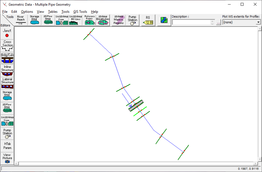
From the main program window, select Edit and then Geometric Data and the river system schematic of Spring Creek will appear, as shown in the figure below. A river reach was drawn and the river was labeled as "Spring Creek" and the reach was titled "Culvert Reach." This river reach was initially defined from the surveyed information to contain 9 cross sections, with river mile 20.535 as the upstream cross section and river mile 20.000 as the downstream cross section. The river station 20.208* was interpolated for this example, and will be discussed in a subsequent section. Additionally, a culvert is displayed which was inserted at river station 20.237 during the procedure of this example.

River System Schematic For Spring Creek

Cross Section Geometry

To enter the cross section data, from the Geometric Data Editor, the Cross Section icon was selected. This activated the Cross Section Data Editor, as shown for river station 20.238 in the figure below. A description of the section was entered as "Upstream end of Culvert" and the X-Y coordinates were entered in the table on the editor. On the right side of the editor, the reach lengths to the next downstream section (cross section 20.227 for this example) were entered as 57 feet for the LOB, main channel, and ROB. For this cross section, the Horizontal variation in n values was selected from the Options menu. This created an additional column in the X-Y coordinates section in which the Manning's n values were entered at the locations along the width of the cross section where the n values change. For this specific cross section, the n values only changed at the left and right over bank locations. Therefore, this horizontal variation option was not necessary. The n values could have been entered directly on the right side of the data editor in the LOB, Channel, and ROB fields. This option was merely selected to display this possibility.

Cross Section Data Editor

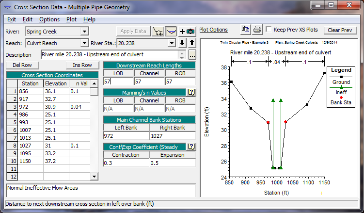
Additionally, on the right side of the data editor, the left and right stations of the main channel were entered. For this cross section, the left side of the main channel is defined to start at station 972 and end at the right station of 1027 feet. Finally, the contraction and expansion coefficients were entered as 0.3 and 0.5, respectively. These coefficients are used by the program to determine the energy losses due to the flow contracting or expanding as it travels from one cross section to the next. Typical values of these coefficients for gradual transitions are 0.1 and 0.3 for contractions and expansions, respectively. However, at locations where there are sudden changes in the cross section geometry (i.e., flow into or out of a culvert or bridge opening), the coefficients may take larger values. The selection of these coefficients is discussed in detail in Chapter 3 of the Hydraulic Reference Manual. For this cross section (being the section immediately upstream of the culvert opening), the coefficients were initially selected as 0.3 and 0.5 for the contraction and expansion, respectively. After the flow analysis, ranges for these values were determined by using the methods outlined in the HEC-1995 research document. These ranges were compared to the selected values and will be discussed near the end of this example.

The cross-section information for the other river stations were entered in a similar fashion as for river station 20.238. Finally, the ineffective flow areas of the cross sections were entered. This option allows the user to define areas of the cross section that will contain water but the water is not flowing in the downstream direction. This option is typically used at cross sections in the vicinity of a culvert or bridge. For this example, the ineffective flow option was used at river station 20.238 (located immediately upstream of the culvert) and at river station 20.227 (located immediately downstream of the culvert).

From the Cross Section Data Editor, select River Station 20.238, Options, and then Ineffective Flow Areas. This will display the Ineffective Flow Editor shown in the top figure below. River station 20.238 was surveyed at a location 5 feet upstream from the culvert. Typically, the stationing of the ineffective flow areas are set on a 1:1 ratio to the distance from the opening. When the culvert data are entered, the centerline stations of the two culverts will be 996 and 1004 feet and each culvert will be 6 feet in diameter. Therefore, the left edge of the opening is at station 993 and the right edge is at station 1007. Using the 1:1 ratio, the left ineffective flow station was set to be equal to 5 feet left of the left opening. Similarly, the right ineffective flow station was set to be equal to 5 feet right of the right side of the openings. These values were entered as 988 and 1012 feet for the left and right stations, respectively. Finally, the elevation of the ineffective flow area was set to be equal to 33.7 feet, a value slightly lower than the high cord on the upstream side of the roadway. Similarly, ineffective flow areas were set at cross section 20.227 at stations of 991 and 1009 (since this cross section was only 2 feet downstream of the culvert outlet) and at an elevation of 33.3 feet. The location of these ineffective flow areas will be discussed further during the analysis of the output. Typically, the culvert information may be entered first and then the modeler can enter the location of the ineffective flow areas more readily with the location of the culverts known.

Cross Section Placement

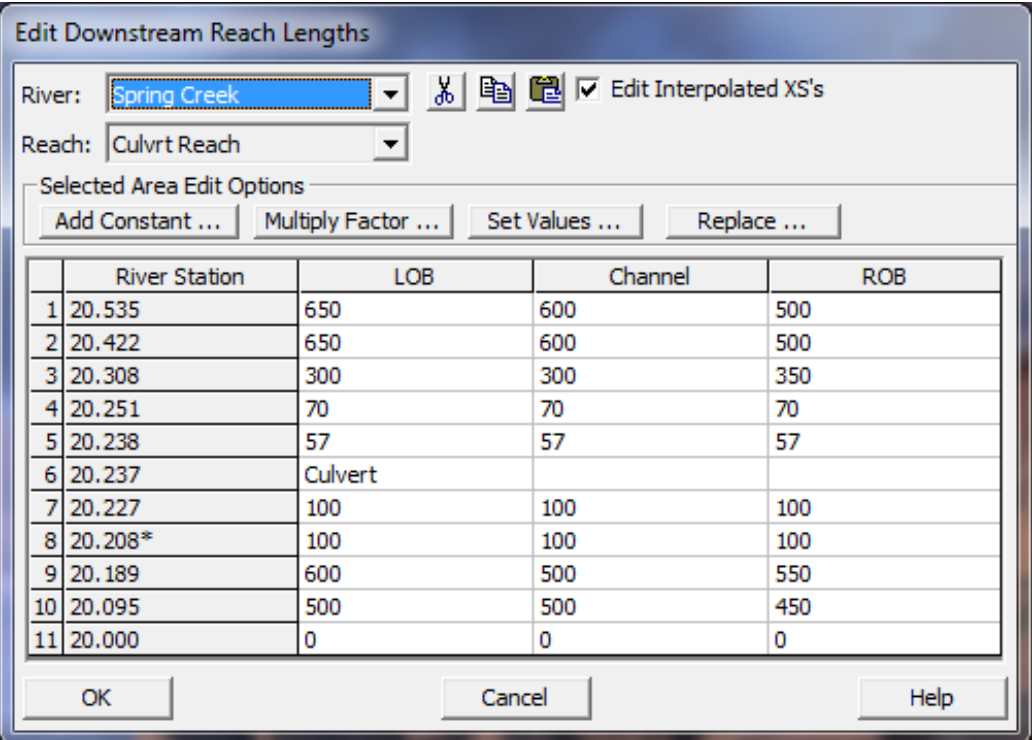
From the Geometric Data Editor, select Tables and then Reach Lengths. This will display the table shown in the bottom figure below. This displays the initial placement of the cross sections as obtained from the field data available for the analysis. (The figure does not show the inclusion of river station 20.208* which will be added subsequently.)

Reach Lengths Table For Spring Creek

The placement of the cross sections relative to the location of the culvert is crucial for accurate prediction of expansion and contraction losses. The culvert routine (as does the bridge routine) utilizes four cross sections specifically located on both sides of the structure to determine the energy losses through the culvert. (Additionally the program will interpret two cross sections inside of the culvert by superimposing the culvert and roadway data onto both the immediate downstream and immediate upstream cross sections from the culvert.) The following is a brief summary for determining the locations of the four cross sections. This procedure is identical to the procedure used for determining the cross section locations for a bridge analysis. The modeler should review the discussion in Chapter 6 of the User's Manual and Chapter 6 of the Hydraulic Reference Manual for further discussion.

First Cross Section. Ideally, the first cross section should be located sufficiently downstream from the culvert so that the flow is not affected by the structure (i.e., the flow has fully expanded). This distance, referred to as the expansion length (Le), should be determined by: field investigation during high flows; the procedure outlined in a recent study by the USACE \[HEC-1995\]; or other acceptable procedure. For this example, the criteria developed by USACE \[HEC-1995\] research document was utilized to determine the expansion reach length. To utilize this method, an initial length was estimated from values obtained in tables that are presented in the document and provided in Appendix B of the Hydraulic Reference Manual. Then, after the flow analysis was completed, the location was evaluated based on equations developed from the research. (This evaluation will be discussed near the end of this example.)

First, the following criteria were required to determine the location of the first cross section:

$\begin{array}{l}n_{ob}/n_c=0.1/0.04=2.5 \\ b/B = 14/145 = 0.10 \\ S = (0.20/200) \cdot 5280=5.28 \ ft/mile \\ L_{obs}= \left[ \left( 993-925\right) + \left( 1070-1007 \right) \right] /2 = 70 \ ft\end{array}$

where :

$\begin{array}{l}n_{ob}\end{array}$ = Manning's n value for the overbank at cross section 20.251
$\begin{array}{l}n_c\end{array}$ = Manning's n value for the main channel at cross section 20.251
$\begin{array}{l}b\end{array}$ = culvert opening width, ft (m)
$\begin{array}{l}B\end{array}$ = total floodplain width, ft (m)
$\begin{array}{l}S\end{array}$ = slope, ft/mile
$\begin{array}{l}L_{obs}\end{array}$ = average length of the side obstruction, ft

Substitution of the field data yields the results as shown above. With these values, the expansion ratio (ER) was determined to range from 0.8 to 2.0 from Table B-1 in Appendix B of the Hydraulic Reference Manual. The expansion ratio (ER), is the length of expansion (Le) divided by the average length of obstruction (Lobs). For this example, an average value of 1.4 was initially used for the expansion ratio. Therefore, the expansion reach length will be the expansion ratio times the average length of obstruction:

$\begin{array}{l}\displaystyle L_{e} = \left(ER \right) \left(L_{obs} \right) = \left( 1.4 \right) \left(70 \right) = 100 ft\end{array}$

From the initial values of the cross section locations, the expansion reach length is the distance from cross section 20.227 to 20.189. This distance is initially set at 200 feet. From the above analysis, it was determined that the distance should be approximately 100 feet. Therefore, an additional cross section was placed 100 feet downstream from cross section 20.227.

To produce this cross section, field data should be utilized. If this data is not available, then the program has the ability to interpolate a cross section. From the Geometric Data Editor, Tools, XS Interpolation, and then Between 2 XS's were selected. "Culvrt Reach" was selected as the river reach (the only reach in this example) and river station 20.227 was entered as the upper river station (this will default to river station 20.189 as being the lower river station). The maximum distance between the interpolated cross sections was set to be 100 feet and then the interpolation was performed. This resulted in the display shown in the figure below. For additional information on cross section interpolation, refer to Chapter 4 of the Hydraulic Reference Manual and Chapter 6 of the User's Manual. The interpolation window was closed and the river schematic displayed the new interpolated cross section at river station 20.208* (as shown in the first figure on this page). The number 20.208 was the default setting since the distance chosen (100 ft) was equal to one half the previous reach length (200 ft).

Cross Section Interpolation

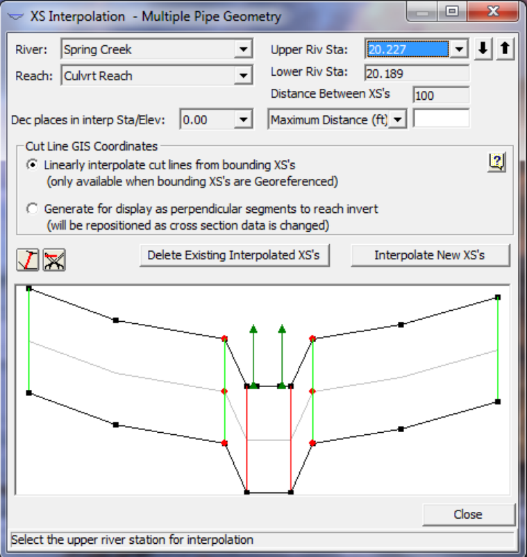
After interpolating the new river station, from the Geometric Data Editor Tables and then Reach Lengths were selected. This resulted in the table shown in the preceding figure except that the interpolated cross-section 20.208* appeared and the distances from cross section 20.227 to 20.208* were 100 feet and from 20.208* to 20.189 were also 100 feet for the LOB, channel, and ROB. The program now considered cross section 20.208* as being the location of the fully expanded cross section.

Second Cross Section. The second cross section used by the program to analyze the energy losses through the culvert is located within a few feet downstream of the structure. This section should be close to the culvert (within a few feet) and reflect the effective flow area on the downstream side of the culvert. Therefore, any ineffective flow areas outside of the flow expanding out of the culvert, should not be used for conveyance calculations. For this example, cross section 20.227 was located two feet downstream from the culvert. The ineffective flow areas were developed previously using this distance. Finally, after the culvert and roadway geometry were entered, the program superimposed the geometry onto this cross section to develop a cross section inside the culvert at the downstream end.

Third Cross Section. The third cross section is located within a few feet upstream from the culvert and should reflect the length required for the abrupt acceleration and contraction of the flow that occurs in the immediate area of the opening. Similar to the second cross section, this cross section should also block the ineffective flow areas on the upstream side of the culvert. For this example, cross section 20.238 was located five feet upstream of the culvert. Similar to the second cross section, the program will superimpose the culvert geometry onto the third cross section to develop a cross section inside the culvert at the upstream end.

Fourth Cross Section. The fourth cross section is located upstream from the culvert where the flow lines are parallel and the cross section exhibits fully effective flow. The distance between the third and fourth cross section, referred to as the contraction reach length, can be determined by: 1) field investigation during high flows, 2) the procedure outlined in a recent study by the USACE \[HEC-1995\]; or 3) other acceptable procedure. For this example, the criteria developed by USACE \[HEC-1995\] research document was utilized to determine the contraction reach length. To utilize this method, an initial length was estimated from values obtained in Table B.2 in Appendix B of the Hydraulic Reference Manual. To use this method, the following criteria were necessary:

$\begin{array}{l}n_{ob}/n_c = 0.1/0.04 = 2.5 \\ S = 0.2/200 \cdot 5280 = 5.28 \ ft/mile\end{array}$

where the variables are as described previously. Substitution of the values yields the results as shown above. With these values, the contraction ratio (CR) was determined to range from 0.8 to 1.5 from Table B-2. The contraction ratio is the length of contraction (Lc) divided by the average length of obstruction. For this example, an average value of 1.15 was used for the contraction ratio. Therefore, the contraction reach length will be the contraction ratio times the average length of obstruction:

$\begin{array}{l}\displaystyle L_c = \left(CR \right) \left( L_{obs} \right) = \left( 1.15 \right) \left( 70 \right)= 80 \ ft.\end{array}$

From the initial values of the cross section locations, the contraction reach length is the distance from cross section 20.251 to 20.238. This distance was initially set at 70 feet. From the above analysis, it was determined that the distance should be approximately 80 feet. Because these values are so close together, the initial value of 70 feet will be maintained. Finally, after the flow analysis was performed, the location of this cross section was evaluated and will be discussed near the end of this example.

Culvert Data

From the Geometric Data Editor, the Bridge/Culvert icon was selected. This activated the Bridge Culvert Data Editor. To enter the culvert data, Options and then Add a Bridge and/or Culvert were first selected. The location for the culvert was entered as 20.237. Then, the bounding river stations (20.227 and 20.238) appeared on the Bridge Culvert Data Editor. Next, the deck/roadway data and then the culvert geometric data were entered. Each of these are discussed in the following sections.

Deck/Roadway Data. To enter the data for the deck/roadway, the Deck/Roadway icon on the left side of the Bridge Culvert Data Editor was selected. This activated the Deck/Roadway Data Editor as shown in the figure below. Along the top row of the deck/roadway data editor, the user must first enter the distance from the upstream side of the deck/roadway to the cross section that is placed immediately upstream of the culvert (cross section 20.238 for this example). This distance was set at 10 feet. The next field is the width of the roadway. For this example, this distance was 40 feet. The program will then add the 10 feet and the 40 feet to obtain 50 feet as the distance from cross section 20.238 to the downstream end of the deck/roadway. From the cross section geometric data, the distance from cross section 20.238 to 20.227 was 57 feet. This allowed for 7 feet of distance from the downstream side of deck/roadway to cross section 20.227.

The final field along the top row is the weir coefficient. This coefficient is used when the flow overtops the roadway and weir flow occurs. For this example, a value of 2.6 was selected as the weir coefficient for the roadway. This value may be changed to account for the shape of the roadway and the degree of obstructions along the edge of the roadway. Additional information on weir flow is presented in Chapter 6 of the Hydraulics Reference Manual.

Deck/Roadway Data Editor

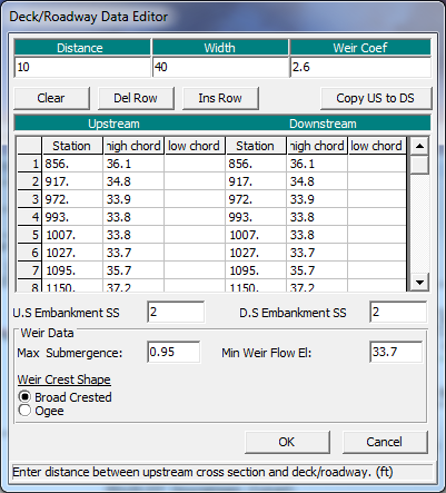
The central portion of the editor consists of fields to enter the stations and elevations of the deck/roadway. The values for this example are as shown in the figure. If the upstream and downstream decking is identical, then the user needs to only enter the upstream information and then select Copy Up to Down. (Note: For culverts, only the high cord information is required. The program will automatically block out the area between the high cord and the ground. For a bridge analysis, the low cord information is required to define the bridge opening. For a culvert analysis, the culvert data will define the openings below the high cord for the locations of the culverts.)

The next two fields are the US and DS Embankment Side Slopes. These values were entered as 2 (horizontal to 1 vertical). For a culvert analysis, these values are only used for the profile plot.

The bottom of the editor consists of three additional fields. The first field is the Maximum Allowable submergence ratio. This is the ratio of downstream flow depth to upstream energy, as measured from the minimum high cord of the deck. When this ratio is exceeded for a bridge analysis, the program will switch from the weir flow equation to the energy method to determine the upstream flow depth. For a culvert analysis, this ratio is not used because the program cannot perform a backwater analysis through a culvert flowing full. Therefore, the weir analysis method will always be used when overflow occurs.

The second field is the Minimum Weir Flow Elevation. This is the elevation that the program uses to determine when weir flow will begin. If this field is left blank, the program will use the lowest value of the high cord on the upstream side of the deck. Alternatively, the user can enter a value for the program to start checking for the possibility of weir flow. For this example, an elevation of 33.7 feet was used. This is the elevation of the roadway above the culvert openings on the upstream side of the culvert. (Note: This is also the minimum elevation of the high cord and therefore, this field could have been left blank.)

Finally, the last field requires the selection of the weir crest shape: broad crested or ogee shaped. This selection is used for the type for submergence correction. For this example, a broad crested weir shape submergence correction was used. With all of the data entered, the OK button was selected to exit the Deck/Roadway Data Editor.

Culvert Geometric Data. To enter the culvert geometric data, from the Bridge Culvert Data Editor, the Culvert icon was selected. This activated the Culvert Data Editor as shown in the figure below. Each of the fields for the editor are described in the following sections.

Culvert ID - By default, the identifier for the first culvert will be set to "Culvert #1." A culvert type is defined by the shape, diameter (or rise and span), chart number, scale, length, n value, loss coefficients, upstream invert, and downstream invert. If all of these parameters are the same for each culvert, then the modeler will only have one culvert type. Then the modeler can enter up to 25 identical barrels for this culvert type, with each barrel occurring at a different location (defined by the upstream centerline and downstream centerline). If any of the culvert parameters change, then the modeler must define each culvert that is different as a separate type (to a maximum of 10 culvert types at the same river station), with each type containing up to 25 identical barrels. For this example, the culvert consisted of only 1 culvert type (since all of the parameters were the same for each barrel) but it contained two identical barrels (with each placed at separate upstream and downstream centerline locations).

Solution Criteria - The user has the option to select to use the result for inlet control or outlet control as the final answer for the upstream energy grade line value. The default method is to use the highest of the two values, as was selected for this example.

Shape - The culvert shape is chosen from the eight available shapes: circular, box, elliptical, arch, pipe arch, semi-circle, low arch, or high arch. For this example, the culvert barrels were circular shape. To select the shape, press the down arrow on the side of the shape field and highlight the desired shape.

Culvert Data Editor

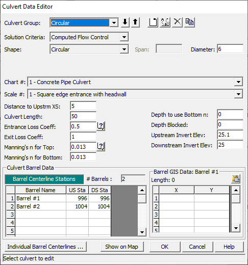
Diameter, Rise, or Rise and Span - Depending on the shape of the culvert, the modeler must enter the inside dimensions of the culvert. For a circular pipe, only the diameter is required. For other shapes, the rise is defined as the inside vertical measurement and the span is the inside horizontal measurement. (Note: For box culverts with chamfered corners, refer to the discussion in Chapter 6 of the Hydraulic Reference Manual.) For this example, the circular culvert was set to have a diameter of 6 feet.

Chart # - Each culvert type and shape is defined by a Federal Highway Administration Chart Number. Depress the down arrow next to this field to select the appropriate chart number. Once a culvert shape has been selected, only the corresponding chart numbers available for that culvert shape will appear in the selections. Descriptions for the chart numbers appear in Chapter 6 in the Hydraulic Reference Manual. For this example, the culvert chart was selected as "1 - Concrete Pipe Culvert."

Scale - This field is used to select the Federal Highway Administration scale that corresponds to the selected chart number and culvert inlet shape. Only the scale numbers which are available for the selected chart number will appear for selection. Descriptions for the scale numbers appear in Chapter 6 in the Hydraulic Reference Manual. The scale for this example was "1 - Square edge entrance with head wall."

Distance to Upstream XS - This is the distance from the inlet of the culvert to the upstream cross section (20.238). For this example, this was a distance of 5 feet. On the Deck/Roadway Data Editor, a measure of 10 feet was entered for the distance from the upstream side of the deck/roadway to the upstream cross section. Therefore, the culvert entrance is located midway between the upstream side of the roadway and cross section 20.238.

Culvert Length - This field is the measure of the culvert (in feet or meters) along the centerline of the barrel. The length of the culvert for this example was 50 feet. The program will add this 50 feet to the 5 foot distance from cross section 20.238 (to the culvert entrance) and obtain 55 feet. The reach length from cross section 20.238 to 20.227 is 57 feet, which leaves 2 feet from the exit of the culvert to the downstream cross section.

Entrance Loss Coefficient - The value of the entrance loss coefficient will be multiplied by the velocity head at the inside upstream end of the culvert to obtain the energy loss as the flow enters the culvert. Typical values for the entrance loss coefficient can be obtained from Tables 6.3 and 6.4 in the Hydraulic Reference Manual. The entrance loss coefficient for the concrete pipe in this example was set at 0.5.

Exit Loss Coefficient - To determine the amount of energy lost by the water as it exits the culvert, the exit loss coefficient will be multiplied by the difference of the velocity heads from just inside the culvert at the downstream end to the cross section located immediately downstream of the culvert exit. In general, for a sudden expansion, the exit loss coefficient should be set equal to 1. However, this value may range from 0.3 to 1.0. For this example, the exit loss coefficient was set to be equal to 1.0.

Manning's n for Top - This field is used to enter the Manning's n value of the top and sides of the culvert lining and is used to determine the friction losses through the culvert barrel. Suggested n values for culvert linings are available in many textbooks and also may be obtained from Table 6.1 in the Hydraulic Reference Manual. Roughness coefficients should be adjusted according to individual judgment of the culvert condition. For this example, a Manning's n value of 0.013 was used for the concrete culvert.

Manning's n Value for Bottom – This field is used to enter the Manning's n value of the bottom of the culvert. For most culverts, this field will be the same as the Manning's n value for the top. However, if the culvert has a natural bottom, or something has been placed in the bottom for fish passage, the n value may vary.

Depth to use Bottom n – This field is used to enter a depth inside of the culvert that the bottom n value is applied to. If the bottom and top n value are the same, a value of zero should be entered.

Depth Blocked – This field is used to fill in a portion of the culvert. The user enters a depth, and everything below that depth is blocked out.

Upstream and Downstream Invert Elevation - These two fields are used to enter the elevations of the inverts. For a particular culvert type, all of the identical barrels will have the same upstream invert elevation and downstream invert elevation. For this example, the upstream invert was set at an elevation of 25.1 feet and the downstream invert was 25.0 feet.

Barrel Centerline Stations - This table is used to enter the name of each barrel, and the stationing (X-coordinates) of the centerline of the culvert barrels. The upstream centerline is based upon the X-coordinates of the upstream cross section (20.238) and the downstream centerline is based upon the X-coordinates of the downstream cross section (20.227). This example employs two culvert barrels, with the centerline of the barrels occurring at stations 996 and 1004 feet, as measured on both cross sections. For this example, the X-coordinate geometry of both cross section 20.238 and cross section 20.227 are referenced from the same left station starting point. Therefore, the upstream and downstream centerline stations are the same value and this will align the culvert in the correct configuration as being parallel to the channel. The modeler must be cautious to ensure that the centerline stationing of the culvert ends align the culvert in the correct position.

# Barrels - This field will automatically display the number of barrels entered by the user (determined by the number of centerline stations entered). Up to 25 identical barrels can be entered for each culvert type, and this example consisted of 2 identical barrels.

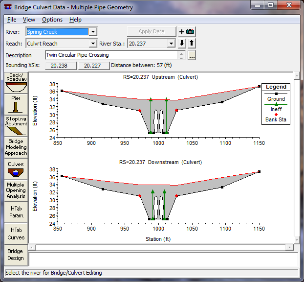
This completed the necessary geometric data for the analysis. The OK button at the bottom of the Culvert Data Editor was selected and this displayed the culvert as shown in the following figure. The geometry data editors were then closed and the geometry was saved as "Multiple Pipe Geometry."

Bridge/Culvert Data Editor For Spring Creek

Steady Flow Data

To perform the steady flow analysis through the culvert, the user must enter the flow data and boundary conditions for each flow profile. Each of these components is discussed below.

Flow Data

To enter the flow data, from the main program window Edit and then Steady Flow Data were selected. This activated the Steady Flow Data Editor as shown in the figure below. For this example, 3 flow profiles were computed. A value of "3" was entered as the number of profiles and the central table of the editor established three columns for the flow profiles. The flow values were then entered at the upstream river station (20.535) as the values of 250, 400, and 600 cfs. Additionally, the profile names were changed to be "5 yr," "10 yr," and "25 yr."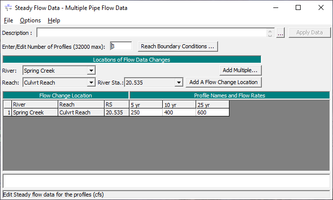
Steady Flow Data Editor

Boundary Conditions

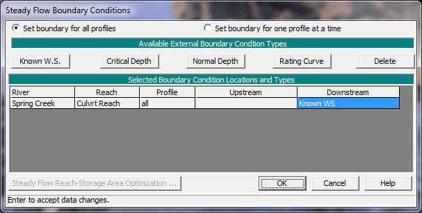
To enter the boundary conditions the Boundary Conditions icon at the top of the Steady Flow Data Editor was selected. This activated the Boundary Conditions Editor as shown in the top figure below. This flow analysis was performed in the subcritical flow regime. Therefore, a boundary condition was established at the downstream end of the reach for each flow profile. For a detailed discussion on the boundary conditions, the modeler is referred to Chapter 7 of the User's Manual and Chapter 3 of the Hydraulic Reference Manual. From the Boundary Conditions Data Editor, the boundary conditions were entered by first selecting the Down Stream field and then Known W. S. This activated the known water surface boundary condition window as shown in the bottom figure.

Boundary Conditions Data Editor

Known Water Surface Boundary Conditions

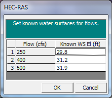
As shown in the bottom figure, a known water surface elevation was then entered for each of the flow profiles that were computed. For this example, the known water surface elevations of 29.8, 31.2, and 31.9 were entered for the flows of 250, 400, and 600 cfs, respectively. Once the data were entered, the OK button was selected to exit this window. This completed the necessary steady flow data for the analysis and the data were saved as "Multiple Pipe Flow Data."

Steady Flow Analysis

To perform the steady flow analysis, from the main program window Run and then Steady Flow Analysis were selected. This activated the Steady Flow Analysis Window as shown in the figure below. A short ID was entered as "Base Plan" and a subcritical flow analysis was selected in the lower left corner of the editor. From the Options menu, the Set Output Options was selected and then an "x" was placed next to Critical Always Calculated. This will cause the program to always calculate critical depth at every cross section. This will add computational time to larger analyses; however, this will enable the user to view the critical flow depth along the river reach.

Additionally, from the Options menu, ensure that there is a "" adjacent to the option Check data before execution. With this option, the program will check to ensure that all pertinent information is present before the analysis is performed. It cannot determine the accuracy of the data. (Note: If there is a check mark next to this option, a selection of this option will remove the check mark.) Finally, the geometry file "Multiple Pipe Geometry" and the steady flow file "Multiple Pipe Flow Data" were saved as the plan "Spring Creek Culverts", with a shirt ID of "Base Plan." Then, the COMPUTE button was selected to perform the steady flow analysis.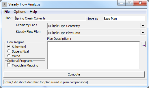 Steady Flow Analysis Window

Output Analysis

For the analysis of the output, the modeler has various options to review the data. For this analysis, evaluations were performed for the expansion and contraction reach lengths and the channel contraction and expansion coefficients. Then, the water surface profiles were reviewed.

Expansion and Contraction Reach Length Evaluation

Initially the reach lengths were determined using table values obtained from the U.S. Army Corps of Engineers' research document \[HEC-1995\] and the cross sections 20.208* and 20.251 were located based on these initial values. The table values provided a range and the average values were initially used. With the program output, the equations developed in the document were utilized to evaluate the locations (and reach lengths) that were selected. The modeler should be aware that the regression equations were developed based on low flow conditions for bridges and the equations may not be practical for analyses of flow through culverts.

Expansion Reach Length. Cross section 20.208* was the interpolated section that was assumed to be at the location where the flow became fully expanded. To evaluate the location of this cross section, the relationship shown as Equation 3-1 was used. Equation 3-1 is applicable when the width of the floodplain and the discharge is less than those of the regression data. The equation is:

$\begin{array}{l}\displaystyle ER = \frac{l_e}{L_{obs}}= 0.421+0.485\left(\frac{F_{20.227}}{F_{20.208^*}}\right)+0.000018Q\end{array}$

where

$\begin{array}{l}ER\end{array}$ = expansion ratio
$\begin{array}{l}L_e\end{array}$ = expansion reach length, ft
$\begin{array}{l}L_{obs}\end{array}$ = average length of side obstruction, ft
$\begin{array}{l}F_{20.227}\end{array}$ = main channel Froude number at the cross section immediately downstream of the culvert (cross section 20.227 for this example)
$\begin{array}{l}F_{20.208^*}\end{array}$ = main channel Froude number at the cross section of fully expanded flow (cross section $\begin{array}{l}20.208^*\end{array}$ for this example)
$\begin{array}{l}Q\end{array}$ = total discharge, ft³/s

(Note: The subscripts used in Equation 3-1 and all subsequent equations reflect the river station numbering for this example.) From the analysis, the Froude numbers at cross sections 20.227 and 20.208*, for the flow of 600 cfs, are 0.32 and 0.14, respectively. Substituting these values into Equation 3-1 yields an expansion ratio of 1.51. This value falls within the range of 0.8 – 2.0 as determined previously from the table values. With this new expansion ratio, the expansion reach length is:

$\begin{array}{l}\displaystyle L_e = \left(ER \right) \left(L_{obs} \right) = \left(1.51\right) \left(70 \right) = 106 \ ft\end{array}$

Additionally, the expansion ratio has a standard error of 0.26. Using the range of the ER from 1.25 (= 1.51 - 0.26) to 1.77 (= 1.51 + 0.26) yields an Le range from 88 to 124 feet to define the 68% confidence band for Equation 3-1. The actual distance from cross section 20.227 to cross-section 20.208* was set at 100 feet. Therefore, the existing expansion reach length seems appropriate. If the existing length had been significantly outside of the range of the calculated expansion reach length, then a second iteration for the placement of the fully expanded cross section and an additional analysis may be warranted. As a final check, the expansion ratio should not exceed 4:1 and should not be less than 0.5:1.

Contraction Reach Length. Cross section 20.251 is located where the flow lines are parallel to the main channel. To evaluate this location, Equation 3-2 from the research document \[HEC-1995\] was utilized. This equation is used when the floodplain scale and dischargers are significantly different than those used in the regression analysis and is:

$\begin{array}{l}\displaystyle CR = 1.4-0.333 \left( \frac{F_{20.227}}{F_{20.208^*}} \right) +1.86 \left(\frac{Q_{ob}}{Q} \right)^2 -0.19\left( \frac{n_{ob}}{n_c} \right)^{0.5}\end{array}$

where

$\begin{array}{l}CR\end{array}$ = contraction ratio
$\begin{array}{l}L_c\end{array}$ = contraction reach length
$\begin{array}{l}Q_{ob}\end{array}$ = discharge conveyed by the two overbanks at cross section 20.251, cfs
$\begin{array}{l}n_{ob}\end{array}$ = Manning's n value for the over banks at cross section 20.251
$\begin{array}{l}n_c\end{array}$ = Manning's n value for the main channel at cross section 20.251

From the analysis of the 600 cfs profile, the flow in the two overbanks at cross section 20.251 is 69.33 cfs and the Manning's n values for the overbanks and main channel at cross section 20.251 are 0.10 and 0.04, respectively. Substituting these values into Equation 3-2 yields a contraction ratio of 0.39. The standard error for this equation is 0.19 which yields a range of the CR from 0.20 to 0.58. From the results cited in the research document, a minimum contraction ratio is 0.3:1 and a maximum ratio is 2.5:1. The calculated average value of 0.39 is very close to the minimum value. If this value is used, the contraction reach length would be:

$\begin{array}{l}\displaystyle L_c = \left(CR \right) \left(L_{obs} \right) = \left(0.39\right) \left(70 \right) = 27 \ ft\end{array}$

This is the median value for the range of 14 to 41 feet (using CR = 0.20 and 0.58, respectively). The actual distance used for the contraction reach length (the length from river station 20.251 to river station 20.238) was 70 feet. For this example, the contraction reach length was maintained at the 70 feet value. However, an additional analysis was performed with the 27 feet contraction reach length and no appreciable difference in the water surface was observed to reflect the necessity for the change of the contraction reach length to 27 feet.

Channel Contraction and Expansion Coefficients

The coefficients of contraction (Cc) and expansion (Ce) are used to determine the energy losses associated with the changes in channel geometry. Initially, in the vicinity of the culvert, the coefficients were set at 0.3 and 0.5 for the contraction and expansion, respectively. Each of these values will be evaluated.

Expansion Coefficient. The expansion coefficient can be obtained from Equation 3-3:

$\begin{array}{l}\displaystyle C_e = -0.09+0.570 \left( \frac{D_{ob}}{D_c} \right) + 0.075 \left(\frac{F_{20.227}}{F_{20.208^*}} \right)\end{array}$

where

$\begin{array}{l}C_e\end{array}$ = coefficient of expansion
$\begin{array}{l}D_{ob}\end{array}$ = hydraulic depth (flow area divided by the top width) for the overbank at cross section 20.208*
$\begin{array}{l}D_c\end{array}$ = hydraulic depth for the main channel at cross section 20.208*

From the analysis of the 600 cfs profile, the hydraulic depths for the overbanks and the main channel are 0.58 and 5.66 feet, respectively. Substitution of the values into Equation 3-3 yielded an expansion coefficient of 0.14. This is the median value and the range of ± 0.2 defines the 95% confidence band for Equation 3-3. For this example, a value of 0.5 was used. The value of the expansion coefficient is generally larger than the value used for the contraction coefficient so the value of 0.5 will remain as the selected value. The regression equation (3-3) was developed for bridges with overbank areas larger than the current example. Therefore, the data for this current example may not be within the range of data used to develop the regression equation. The modeler can perform a sensitivity of this coefficient by changing this coefficient and performing subsequent analyses. For this example, a value of 0.3 was used during a subsequent analysis and no appreciable difference was observed in the resulting water surface.

Contraction Coefficient. From the research document \[HEC-1995\], the contraction coefficient is obtained by first determining the relationship:

$\begin{array}{l}\displaystyle b/B = 14/145 = 0.10\end{array}$

where

$\begin{array}{l}b\end{array}$ = culvert opening width, ft (m)
$\begin{array}{l}B\end{array}$ = total floodplain width, ft (m)

From Table B-3 of Appendix B in the Hydraulic Reference Manual, the recommended contraction coefficient range is 0.3 - 0.5. The value selected for this example was the minimum value of 0.3, which reflects a value in between a typical contraction and an abrupt contraction.

Water Surface Profiles

From the main program window, select View and then Water Surface Profiles. This will result in the display shown in the figure below. In the figure, the water surface elevations and the energy gradelines are shown for all three flow profiles (the variables can be selected from the Options menu). As can be seen in the figure, the first flow of 250 cfs was able to travel through the culvert without submerging the entrance. The second flow (400 cfs) caused the headwater and tailwater to submerge the entrance and exit of the culvert, respectively. Finally, the third flow (600 cfs) caused an overtopping of the roadway, which yielded weir flow.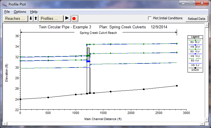 Water Surface Profiles For Spring Creek Culverts

To investigate the first flow profile, from the main window select View, Cross Section Table, Type, and then Culvert. Select the river reach of "Culvrt Reach," river station 20.237, profile 1, and culvert #1. This will display the table shown in the figure below. The left column of the table shows a total flow rate of 250 cfs through the culvert. Since the culvert has two identical barrels, this yields a flow of 125 cfs through each barrel. The table also shows that the normal depth (3.56 ft) was greater than the critical depth (3.02 ft), which corresponds to subcritical flow occurring through the culvert. At the bottom of the left column, the data shows that the culvert did not flow full for any length of the culvert. Additional values such as the velocity in the culvert at the upstream and downstream ends are displayed.

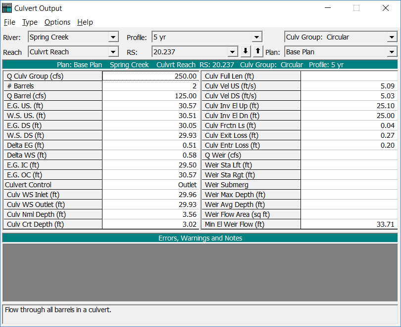
Culvert Tables For Flow equal to 250 cfs

To determine the control of flow through the culvert (i.e., inlet or outlet), the values of the upstream energy grade line necessary for inlet control (E.G. IC) and outlet control (E.G. OC) are shown in the left column of the above figure. For the specified flow of 250 cfs, the upstream energy grade line for inlet control was 29.50 feet and the upstream energy grade line for outlet control was 30.57 feet. The program will select the higher of these two values to determine which type of control will occur (since "Highest Upstream EG" was selected on the Culvert Data Editor). For this example, outlet control occurred and the energy gradeline used by the program is listed as the energy grade line upstream of 30.57 feet. Finally, by using the values in the figure above and following the decision flow chart shown as Figure 6.9 in the Hydraulic Reference Manual, the modeler can determine the procedure used by the program to determine the water surface profile. For this flow of 250 cfs, the program used the Direct Step Method to calculate the water surface profile.

For an analysis of the second flow (400 cfs), a similar procedure can be followed. For this example, the second flow resulted in full flow along the entire length of the barrels of the culvert. The upstream water surface profile was determined by using the FHWA full flow equations.

For the third flow (600 cfs), the inlet and outlet were submerged and weir flow occurred over the roadway. Select the Culvert type Cross Section Table (as performed for the figure above) and select the third flow profile. This will display the table shown in figure below. For this profile, the flow through the culvert was 525.75 cfs, 262.87 cfs through each identical barrel. The energy grade line upstream was calculated to be 34.34 feet, which corresponds to the outlet control energy grade line as shown.

The weir flow at river station 20.237 resulted with a value of 600 - 525.75 = 74.25 cfs. This occurred from an X-coordinate of 945.10 to 1048.77, a distance of 103.67 feet. The main channel bank stations for cross sections 20.227 and 20.238 are at 972 and 1027. Therefore, the weir flow from 945.1 to 972 should balance with the flow in the LOB at river stations 20.227 and 20.238. Additionally, the weir flow from 1027 to 1048.77 should balance with the flow in the ROB at river stations 20.227 and 20.238. At river station 20.237, the amount of weir flow from 945.1 to 972 can be approximated as: the specific length of weir divided by the total weir length times the weir flow. This was calculated as:

$\begin{array}{l}\displaystyle (972.00-945.1)/(103.67)\cdot(74.25) = 19.26cfs\end{array}$

Similarly, the amount of weir flow from 1027 to 1048.77 is approximately 15.4 cfs. Therefore, at river stations 20.227 and 20.238, the flow in the LOB should be approximately 19.26 cfs and the flow in the ROB should be approximately 15.4 cfs.

To determine the amount of flow in the overbanks at cross section 20.227, from the Cross Section Table window, select Type and then Cross Section. Toggle to river station 20.227 for the third flow profile. The values for the flow in the LOB and ROB are zero at this cross section. By toggling to river station 20.238, it was observed that the flows in the LOB and ROB were 36.2 and 34.4 cfs, respectively. Therefore, these flow values in the LOB and ROB for both river stations need to be adjusted to balance with the amount of weir flow.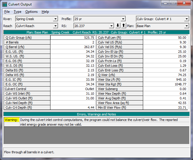
Culvert Table for Adjusted n Values and Ineffective Flow Areas With Flow equal to 600 cfs

The following discussion is provided as an example procedure that can be utilized to balance the weir flow with the overbank flow. The modeler should compare the magnitude of the weir flow to the total flow rate to determine if the procedure is practical for the specific situation.

To adjust the LOB and ROB flow values, first the situation at river station 20.227 was analyzed. Since there was not any flow in the overbanks, the ineffective flow elevation was lowered from 33.3 to 32.0. This will allow for the flow coming over the weir to become active at this downstream cross section. The elevation of 32.0 feet was chosen because it is slightly lower than the calculated water surface (32.01 feet) at river station 20.227. (The user must be cautious not to lower this elevation to a point where the ineffective flow will impact the second flow profile. Each flow profile must be analyzed separately.)

As a second step to balance the weir and overbank flows, at river station 20.238 the Manning's n values in the overbanks were raised from 0.1 to 0.4. Additionally, at river station 20.227, the Manning's n values for the overbanks were decreased from 0.10 to 0.06. Since the n value is inversely proportional to the flow rate, the increase in n value at river station 20.238 will cause a decrease in the flow rate in the overbank areas. Similarly, the decrease in the n value at river station 20.227 will cause an increase in the flow rate in the overbank areas.

After these adjustments were made, the geometry file was saved as "Adjusted Ineffective + n Values." Then this geometry file and the steady flow data file were saved as a plan entitled "Sp. Cr. Culverts - Adj. Weir Flow." The user can activate this plan to review the remaining discussion of the output.

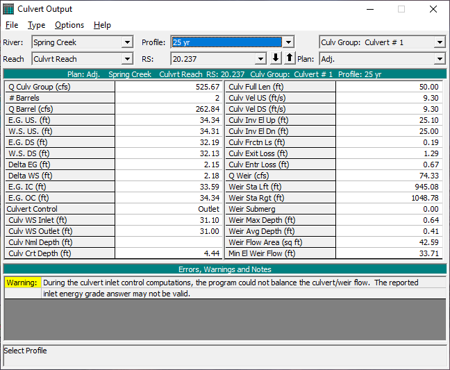
After the adjusted plan was executed, the weir flow at river station 20.237 was determined to be 74.20 cfs, as shown in the Culvert Table of the figure below. This weir flow occurred from X-coordinates of 945.08 to 1048.78, a distance of 103.65 feet. As calculated previously, the approximate portion of this weir flow that occurred from 945.11 to 972 is:

$\begin{array}{l}\displaystyle (972.00-945.08)/(103.7)\cdot (74.32) = 19.29cfs\end{array}$

Similarly, the portion of the weir flow from 1027 to 1048.78 was approximately 15.6 cfs. These flow values were then compared to the flow values in the LOB and ROB at river stations 20.227 and 20.238.

At river station 20.227, the flow in the LOB was 6.93 and the flow in the ROB was 5.60 cfs. These values are approximately equal to the portions of the weir flow values as determined above. Therefore, these flow rates were considered as being balanced with the weir flow. If the flows in the overbanks had been higher than the portions of the weir flow, then the Manning's n values in the overbanks at river station 20.227 would have been increased until a balance was achieved.

At river station 20.238, the flow in the left and right overbanks were 9.91 and 9.38 cfs, respectively. These flow rates were considered to be reasonably in balance with the portions of the weir flow. If the flow rates were not in balance, then the n values would have been adjusted further until a balance was achieved.

For both river stations 20.227 and 20.238, it should be noted that the flow rates do not exactly match the portions of the weir flow as calculated above. An exact match is not warranted because the weir flow portions were approximate and the weir flow that contributes to the left and right overbank is only a minor portion of the total flow rate. If observed high water marks were available, the modeler could make adjustments to the data to more accurately predict the actual water surface elevations.

Culvert Table for Adjusted n Values and Ineffective Flow Areas With Flow equal to 600 cfs

For additional detailed analysis of the flow, the modeler should review the energy losses associated with the contraction and expansion of the flow in the channel and the entrance and exit losses for the culvert to evaluate the selected energy loss coefficients.

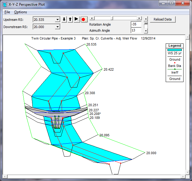
Finally, a three dimensional view of the water surface profiles is displayed in the figure below. This was activated from the main program window by selecting View and then X-Y-Z Perspective Plots. The figure is available to aid the user to view the calculated water surface profiles. The water surface image represents the hydraulic grade line at the respective cross section locations.

3D Perspective Plot of Spring Creek Flow Profiles

Summary

For this example, a culvert was analyzed with three flows. The culvert was composed of two identical circular barrels. During the review of the output, it was determined that initially the flow in the left and right overbanks at the upstream and downstream cross sections from the culvert did not match the weir flow that was occurring. In order to balance the weir flow with the overbank flows, the Manning's n values and the ineffective flow areas were adjusted at the cross sections that bound the culvert.

The next example (Example 4) utilizes this data set and adds another culvert type to the geometric data. This creates a multiple culvert analysis, each with multiple identical barrels.