Urban Modeling - Example 23

This example will demonstrate the use of HEC-RAS to analyze many features often found in urban models, namely, pressurized pipe flow. Subsidiary topics discussed in this example are: how to model pipe connections, drop inlets, minor losses, levee breaches, pump stations, and storage areas. The model used in this example is a portion of a New Orleans Parish system. While the data is from actual studies, the model and the results of this example application do not represent current or future conditions of the system.

Although modeling pressurized pipe flow in HEC-RAS is suitable for most projects, the user should be aware of its limitations. First, drop inlets are modeled in HEC-RAS by using lateral structures or a lateral inflow hydrograph; although this is suitable for some models, it does not fully capture all the details associated with drop inlet structures. Also, modeling pipe junctions with HEC-RAS should be done with caution because although it mimics the energy lost through the junction, its results are general and don't account for many of the details associated with modeling pipe junctions. The modeler is referred to Chapter 16 of the User's Manual and Chapter 4 of the Hydraulic Reference Manual for further discussion and an overview of the hydraulic computations for pressurized pipe flow.

To review the data files for this example, from the main HEC-RAS window, select File and then Open Project. Go to the directory in which you have installed the HEC-RAS example data sets. From the "Applications Guide\Chapter 23 – Urban Modeling" subdirectory, there will be a project titled "Orleans Parish Example Model." Once opened, this will activate the following files:

Plan: "Katrina Existing Conditions"
Geometry:"Orleans Parish – Existing Conditions"
Flow: "Katrina Event"

Example 23 - Urban Modeling.zip

Geometric Data

To view the geometric data for the river system, from the main program window select Edit and then Geometric Data. This will activate the Geometric Data Editor and display the river system schematic as shown in figure below. The schematic gives a visual representation of the geometric elements entered by the user.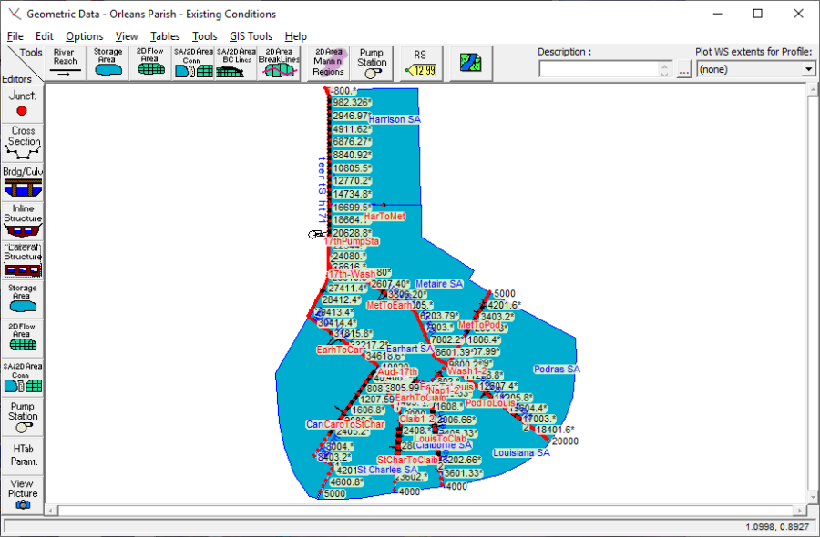

Subsurface Modeling

The subsurface portion of this urban area was modeled with cross sections with lids in order to represent the pressurized pipe system. The pressurized pipe system is directly connected to open channel flow reaches. Additionally, there are several pump stations being modeled, as wells as pipe junctions and bends.

Cross Section Data

The cross section data consists of the X-Y coordinates, Manning's n values, contraction and expansion coefficients, etc. The user can view this data for each river station by selecting the Cross Section icon on the left side of the Geometric Data Editor. Several of the cross sections were interpolated by selecting XS Interpolation from the Tools menu on the Geometric Data Editor.

Open air cross sections were transformed to pressurized pipes by adding a lid to the top of the cross sections. The "pipe" was formed with the cross section as the bottom half of the pipe and the Lid as the top half. This is done by selecting Options and then Add a Lid to XS from the Cross Section Data Editor. A table (as shown in the figure below) will open and the high and low chord elevations and their corresponding station will be entered for each cross section's lid. The lid will be drawn on the cross section diagram of the Cross Section Data Editor once it has been entered and applied.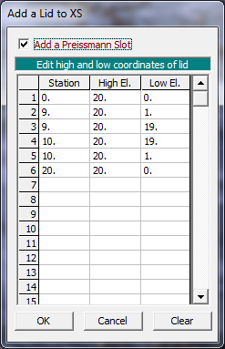Unsteady flow models, such as this one, require that the Add a Preissmann Slot be checked on. The Preissman Slot option can be turned on from each lidded cross section's editor (see figure above) or from a table that shows the locations of all lidded cross sections. This comprehensive table can be viewed by selecting Priessmann's Slot on Lidded XS's from the Tables menu on the Geometric Data Editor. The table is show in the figure below. For more information on Preissmann Slot Theory, the user is encouraged to review Chapter 16 of the User's Manual and Chapter 4 of the Hydraulic Reference Manual.

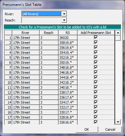
Minor Losses

Minor losses due to bends can be accounted for in HEC-RAS by selecting the Minor Losses feature from the Tools dropdown in the Geometric Data Editor. The Minor Loss Coefficient Editor can be seen in the figure below. A K loss coefficient is required around each bend. The K loss coefficient can vary from 0.0 to 1.0, although the values for bends are usually closer to zero since bend losses typically cause relatively small losses. In this example, each bend's loss value was distributed amongst the bend's surrounding cross sections to represent the fact that bend losses typically occur over a range of pipe and not at one point.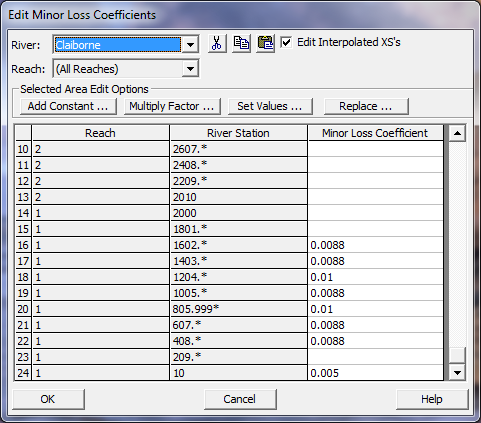

Stream Junction Data

A junction was established by connecting reaches on the river schematic when drawing them. The junction data was added by clicking on the Junct icon from the left side of the Geometric Data Editor. This activated the Junction Data Editor as shown in the figure below. This model consist of 11 junctions, each having a junction length of 10 feet and using the Energy method for steady flow computations and Force Equal WS Elevations for unsteady flow computations.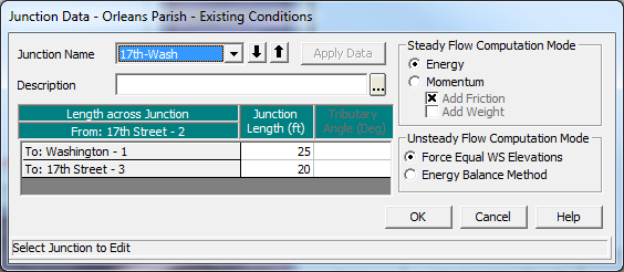

Surface Modeling

The surface flow portion of this urban area is modeled with interconnected storage areas to represent the sheet flow flooding; as well as open channels to represent the surface canal system in this area.

Creating Storage Areas

When creating the storage areas, first the Storage Area icon was selected from the Tools toolbar (not to be confused with the Storage Area icon from the Editors toolbar) of the Geometric Data Editor. The pointer was then placed at the desired location on the river schematic and the storage area was drawn by single clicking and dragging the mouse for each desired point for the storage area. The final point for the storage area was selected by double clicking the mouse. Upon double clicking the mouse, a dialog box appears requesting a storage area name. A name was entered for each storage area created. Points on a storage area may be added or removed by using the Add Points to a Reach or SA and Remove Points to a Reach or SA options found in the Edit menu.

Entering Data for a Storage Area

After the storage area was drawn in the Geometric Data Editor the elevation volume relationship for the storage was established. The data was entered in the Storage Area Editor, displayed in the figure below, which is opened by selecting the Storage Area icon on the Editors toolbar. All the storage areas in this example used the Elevation versus Volume Curve to determine a relationship for calculating storage area. This method was selected by clicking the corresponding radio button and then filling in the elevation volume table listed below it (see below).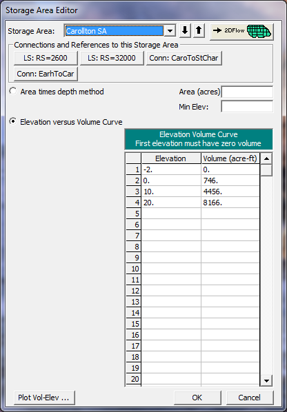

Storage Area Connections

Storage area connections are used to connect storage areas to other storage areas. In this example elevated roadways that divide storage areas are modeled as storage area connections. This feature is used by first selecting the SA/2D Area Connection icon from the Tools toolbar in the Geometric Data Editor. A line can be drawn from one storage area to another by right clicking on the first storage area and then double clicking on the second. A prompt comes up that will ask for the name of the connection. After the user enters a name for the SA connection, it can be selected and edited from the SA/2D Area Connection Editor, which is located on the Geometric Data Editor.

The storage areas that the connector transferred water to and from were selected by pressing the Set SA/2D buttons next to the From and To location fields. The Structure Type was chosen as Weir from the drop down menu for all of the storage area connections. Next the Weir/Embankment icon was selected. The weir width, coefficient, and weir shape were all entered. In addition the weir station and elevations were entered into the table. Both the Connection Data Editor and the Storage Area Connection Weir Data can be seen below.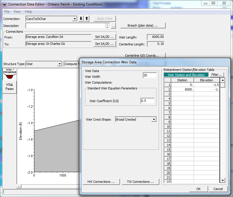

Lateral Structure Connected to a Storage Area

In this example lateral structures were used to model levees or drop inlets. Since HEC-RAS currently does not have a drop inlet feature for modeling a connection between surface flow and sub surface pipe flow, a lateral structure can be used to connect the subsurface pipe system to the surface storage area system. The storage area can be used to represent surface runoff.
In this model, an example of a lateral structure used as a drop inlet is at river station 3600, which connected Reach 2 of Claiborne River to St. Charles SA. This was accomplished by selecting the Lateral Structure icon from the Editors toolbar in the Geometric Data Editor. After selecting the icon, the Lateral Structure Data Editor appears, as shown in the figure below. Once the proper reach and river were selected, under the Options menu, Add a Lateral Structure was selected. The location of the structure was entered at RS 3600. This placed the beginning of the structure between river stations 3602 and 3403.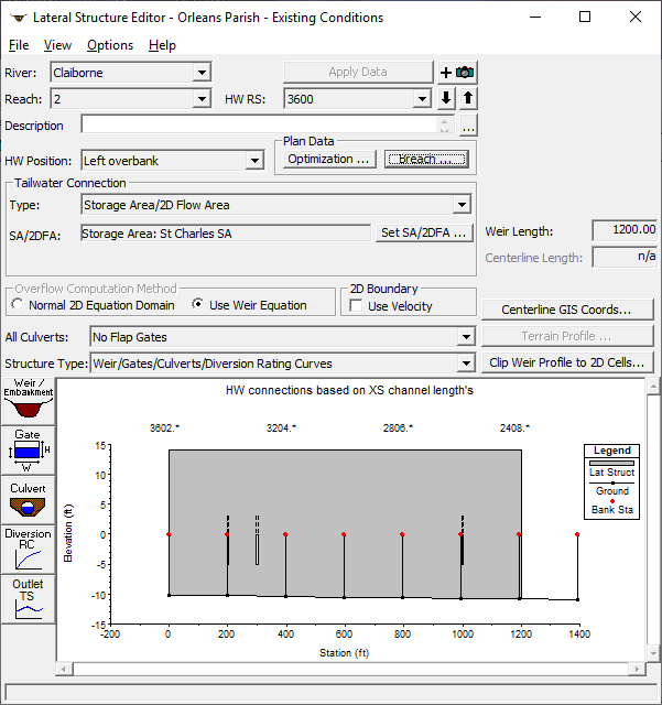To enter data for the structure, the Weir/Embankment icon was selected from the Lateral Structure Data Editor. The data were entered as shown below on the Lateral Weir Embankment Window. The 1200 foot weir is broad crested with a width of 10 feet, placed two feet from the upstream river station 3602 and it has tailwater flow going to a point between two cross sections. The weir flow reference method was chosen as "water surface" and a weir coefficient was established as two.

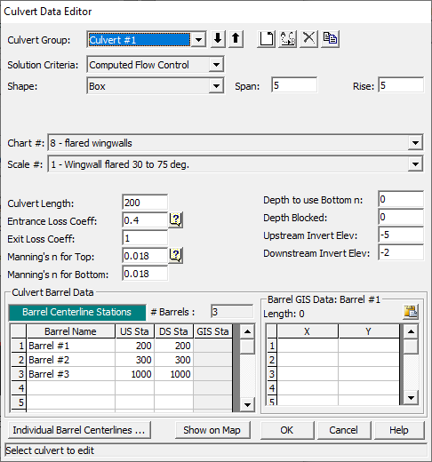
Returning to the Lateral Structure Data Editor, the HW Position was selected as "Left overbank" from the pull-down menu and the Tailwater Connection Type was chosen as Storage Area. Lastly, a connection was made to the storage area by selecting the Set SA/2DFA button. A window then popped up, allowing the user to select a storage area to connect to. On the pull-down menu "Storage area: St Charles SA" was selected.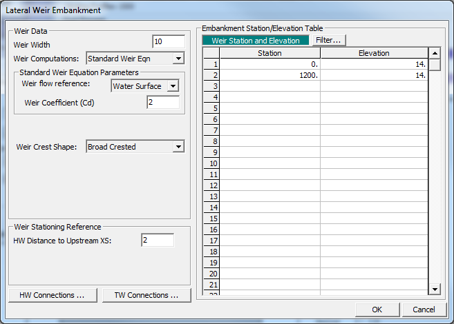The lateral structure at RS 3600 of Claiborne's Reach 2 has culverts along the structure (as do most of the other lateral structures in the system). To enter the data for the culverts, the Culvert icon was selected from the Lateral Structure Data Editor (see second most previous figure). This activated the Culvert Editor and the data was entered as shown in the figure below. Three five by five box culverts were entered at centerline stations 200, 300, and 1000. The culverts were identical, each having a length of 200 feet and flared wingwalls. No flap gates were used at this lateral structure. For more information on entering culverts the user is encourage to review examples 3 or 4 and Chapter 6 of the User's Manual.

Levee (Lateral Structure) Breach Data

Several of the lateral structures in this model were used to represent levees. Once the levee is overtopped, the flow going over the top of the levee is calculated using the weir equations. Modeling the levees as lateral weirs also has the advantage of allowing the user to model a levee breach. The 17^th Street levee (lateral structure) on Reach 2 at RS 16500 was the only structure to be breached in this model.  The breach data is entered from the Lateral Structure Editor (as shown below) by clicking the Breach button under the heading Plan Data. Once clicked, a window will appear titled "Levee (Lateral Structure) Breach Data" as seen in the figure below. First, the option Breach This Structure was checked on. Next, the remaining fields were entered. The levee breach was modeled with a piping failure mode, which was triggered at a water surface elevation of 11.2 feet. A description of each of the fields for the editor is described in Chapter 8 of the User's Manual. Once all the breach data is entered, the breach area is displayed on the lateral structure in the Breach Plot.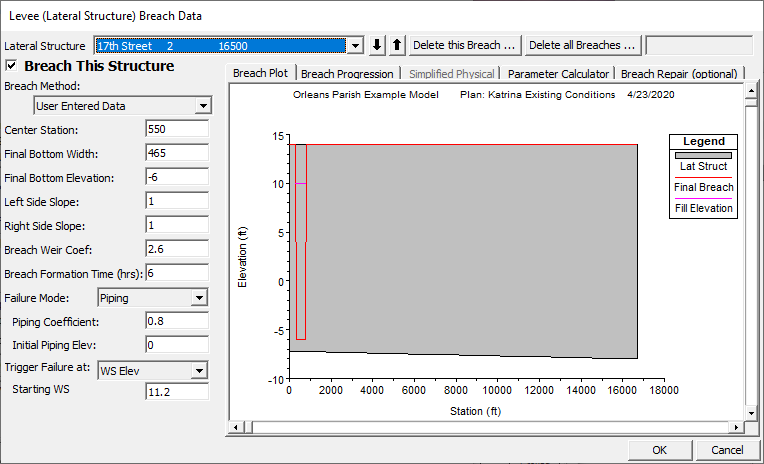

The Breach Progression tab was chosen next and a one-to-one linear relationship was established between the breach time and the breach completion by clicking Set to Linear. Alternatively, Sine Wave could have been selected, giving the breach completion/time relationship a sine correlation.

Lastly, the optional Breach Repair tab was selected from the Levee (Lateral Structure) Breach Data Editor. This option allows the user to signify that the levee will be repaired during the course of the simulation, thereby altering the lateral structure's geometry and unsteady flow calculations. The three fields that must be filled in by the user if selected are: Number of hours after full breach to start repair, Total repair time (hours), and Final filled in elevation. For this example, the fields' values were 48 hours, 24 hours, and 10 feet, respectively.

Inline Structure

An inline structure was used in this data set to represent the 17^th street canal pump station. To add an inline structure, the Inline Structure icon was selected from the left side of the Geometric Data Editor. This activated the Inline Structure Data Editor as shown in the figure below. River "17^th Street" and Reach "2" were chosen, then, Options and Add an Inline Structure were selected and river station 21150 was entered as the location for the weir. The schematic then displayed the cross section data for the river station immediately upstream of the weir location - river station 21200 for this example.

After entering a brief description, a pilot flow of 1 cfs was entered directly beneath the Description field. The Pilot Flow field sets a minimum flow release from the structure, thereby allowing the user to ensure that the weir is always passing flow downstream, even in low flows. In HEC-RAS, no cross section in the model can go dry during the simulation. While there can be zero flow at the structure, the upstream and downstream cross sections must always have water in them. The pilot flow is a simple way to ensure that there is always some minor flow going through the structure.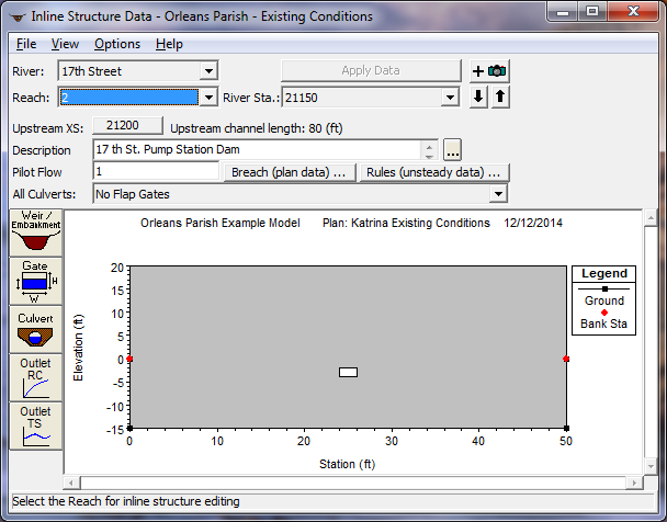Next the weir data was entered. To enter the data for the weir, the Weir/Embankment icon was selected from the left side of the Inline Structure Data Editor. This activated the Inline Structure Weir Station Elevation Data Editor as shown in the figure below. This editor is similar to the deck/roadway editor used for bridges and culverts.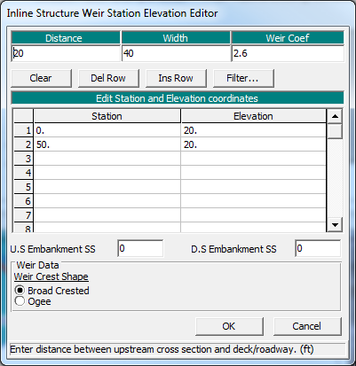The top row of the editor consists of three data entry fields. For the first field, the user must enter the Distance from the upstream cross section (RS 21200) to the upstream side of the weir. For this example, this distance was 20 feet. Next, the Width of the weir was entered as 40 feet. This is a total distance of 60 feet. The distance from river station 21200 to 21120 is 80 feet. Therefore, the distance from the downstream end of the weir to cross-section 21120 is 20 feet. The last field in the top row of the editor is the Weir Coefficient and was entered as 2.6, coinciding with the Broad Crested weir shape chosen at the bottom of the editor.

The central portion of the editor consists of a table in which the user must enter the station and elevation data for the weir. The first station of the weir was entered as zero and the last station is at 50 feet – both have an elevation of 20 feet. With these weir stations and elevation, the program will block out the entire area below the weir crest.

The inline structure has one gate. To enter the data for the gates, the Gate icon was selected from the Inline Structure Data Editor (shown below) which activated the Gate Editor. The Gate type (or methodology) was left at the default of "Sluice" from the pull down menu. The Orifice Coefficient, Weir Shape, Head Reference, and Weir Coefficient were also kept at their default values (0.8, Sill (Invert), Broad Crested, and 3, respectively). The Sluice Discharge Coefficient was set to 0.6. The gate was set with a centerline station of 25 and an invert of -4 feet. It was 2 feet in height and width. The OK button was selected at the bottom of the Gate Editor and the gates appeared on the Inline Structure Data Editor as shown in the figure below. The Inline Structure Data Editor was then closed.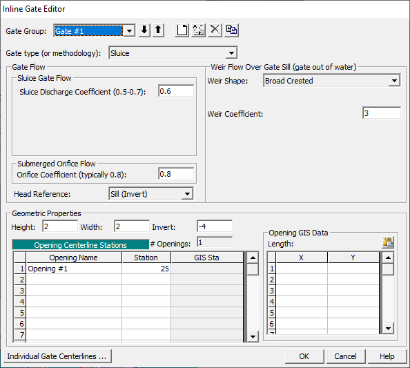

Pump Station

A pump station is used in this example to move water from the 17^th St. Pump Station sump to the outflow canal on the same reach. A pump was added by selecting the Pump Station drawing tool at the top of the Geometric Data Editor. Once the button was pressed, the mouse icon changed to a set of cross hairs with a pump. The pump was placed to the left of the dam and given the name "17thPumpSta" when prompted for a name.

Next, the Pump Station editing tool was selected from the left of the Geometric Data Editor. The Pump Station editor appeared as in the figure below. There are three tabs on the pump station editor, the first is for the pump connection data, the second is for the pump group data, and the third is for the applying advanced rule controls over the pump station. A detailed description of each field within these tabs can be found in Chapter 6 of the User's Manual.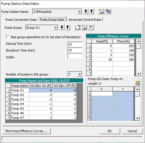The Pump Connection Data was entered first. This was done by clicking the button Set RS adjacent to the Pump From field. Once selected, "17^th Street", "2", and "21392" were selected from the River, Reach, and River Station dropdown menus, respectively. OK was clicked and the Pump To field was set in a similar manner so that the pump released its water downstream to RS 20628.8.

The Pump Group Data was then entered by selecting the second tab. There is only one pump group in this data set; therefore, no additional groups needed to be added. Adding, deleting, and renaming pump groups can be done at the top of the editor using the buttons labeled as such (See the figure above). The Number of Pumps in Group was selected as 7 from the drop down menu. The pump Startup and Shutdown times were both set to 15 minutes. Each pump was then given a water surface elevation in which the each pump was designated to turn on or off. The Pump Efficiency Curve head and flow values were then entered as seen in the figure below. The head represents the total head in the system, which is typically the difference in the water surface elevations between the "from" and the "to" location; however, in HEC-RAS the relationship between head difference and flow should already account for all energy losses in the pump line (friction, bends, junctions, etc…). The rated pump curve from the manufacturer could not be entered because it didn't account for losses. The pump curve used in HEC-RAS was derived by subtracting all energy losses from the manufacturer's pump efficiency curve. The pump efficiency curve was then plotted for visual inspection by pressing the Plot Pump Curves button at the bottom of the window.

Lastly, the Advanced Control Rules tab was selected. This optional tab allows the user to specify rules that will override the physical pump data. Pressing the Add New Rule button opened a window that had six different rule types to choose from: Always apply this rule; Apply based on target flow; Apply based on target WS; Apply based on day/hour; Apply based on day/hour and flow; and Apply based on day/hour and WS. More details on each type can be found in Chapter 6 of the User's Manual. For this example, a new rule was created using the Apply based on day/hour type that restricted the maximum flow rate leaving the pump station to 100 cfs starting at noon on August 29 until zero hundred hours September 30. The transition time was set to 10 minutes. The transition time can allow for a smoother and more stable change in pumping rates.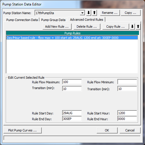

Cross Section Hydraulic Table Parameters

In HEC-RAS, cross sections are processed into tables of elevation versus hydraulic properties of areas, conveyances, and storage. The user is required to set an interval for spacing the points in the cross-section tables. In the Geometric Data Editor the icon Htab Parameters was selected under the Editors toolbar. This displays the Cross Section Table Parameters Window shown in the figure below. The starting elevation, table increment, and number of points columns are automatically filled by the program but may be changed by the user. The program automatically starts the table for each cross section 1 foot above the channel invert. The program chooses a table increment and number of points by first attempting to use 20 points, and choosing an increment that will put the table up to the top of the cross section. If this results in too large of an increment (greater than 1.0 foot) the program will use a one foot increment and add additional points to get the table to the top of the cross section. The increment for this example was set to 1 for "All Reaches" by highlighting the increment column and selecting the Set Values button. The user can set individual values for each cross section if it is deemed necessary. Warning: Always ensure that your cross section tables encompass the complete range of stages that will be modeled. If the tables do not go up to a high enough elevation, the program will have to extrapolate during the computations. More often than not, the extrapolation causes instabilities in the results. To visualize the extent of the tables, a graphic of individual cross sections is shown on the right hand side of the window. The graphic displays the cross section corresponding to the row in which you cursor lies in the table.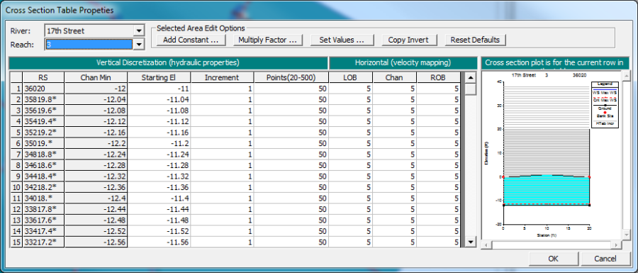

Unsteady Flow Data

The user is required to enter boundary conditions to describe the event, and initial conditions for the system at the beginning of the simulation period. For additional information on unsteady flow data refer to Chapter 8 of the User's Manual, Performing an Unsteady Flow Analysis. The Unsteady Flow Data Editor, shown below, was selected from the main program window under the Edit menu.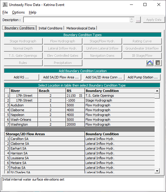

Boundary Conditions

Boundary conditions are required for the farthest upstream and downstream cross sections of the river system. Upon entering the Unsteady Flow Data Editor the farthest upstream and downstream cross sections will automatically be located in the boundary conditions column. In addition, features such as gated inline structures, which also require a boundary condition, will automatically be populated in the Boundary Condition table. In this example there are 15 total boundary conditions: five upstream BC, one downstream BC, and nine internal BC (eight of which are for storage areas).

Boundary conditions are set by highlighting the adjacent cell under Boundary Condition Type. When a cell is highlighted, not all boundary conditions are available. The program will automatically gray out all irrelevant boundary condition types. Internal boundary conditions may be added by selecting one of the buttons under the "Add Boundary Condition Location" heading.

Upstream Boundary Conditions

Flow hydrographs were selected for the six upstream boundary conditions by highlighting the Boundary Condition cell and pressing the Flow Hydrograph button. The window where the Flow Hydrograph is entered is shown in the figure below. The user may select to read hydrograph data from a DSS file or manual enter the data. For further instruction on using a DSS file see Unsteady Flow Application Example 17. For this example the flow hydrograph was manually entered by selecting the Enter Table radio button. The Data Time Interval was set to one hour and the radio button Use Simulation Time was selected causing the initial propagation of the hydrograph to coincide with the beginning of the simulation time window. The hydrograph was then manually entered into the table.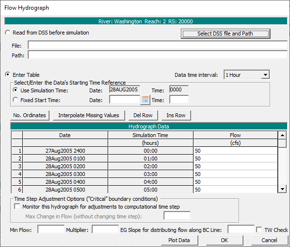

Downstream Boundary Condition

The boundary condition selected for River Station -1000 of 17^th Street, Reach 2 was a stage hydrograph. This stage hydrograph was used to represent the storm surge that occurred inside of Lake Ponchartrain during Hurricane Katrina. Again, the corresponding cell for that particular river station was highlighted and then the Stage Hydrograph button was selected. A window appears that looks nearly identical to the flow hydrograph editor; however, stage values are entered instead of flows. The data time interval was set to one hour and the starting time reference was selected as the simulation time. The stage values were manualyl entered in the Hydrograph Data

Internal Boundary Conditions

Boundary conditions were entered for the gate of the inline structure and the storage areas. The inline structure (RS 21150 of 17^th Street, Reach 2) utilized "T.S. Gate Openings" while the storage areas used a "Lateral Inflow Hydrograph." These boundary condition types were selected in the same manner as the upstream and downstream boundary condition types were selected.

All of the internal boundary conditions used a one hour data time interval and its start time coincided with the simulation time. The gate opening height and the lateral inflow were then manually entered into their respective tables. An example of each boundary condition type can be seen below.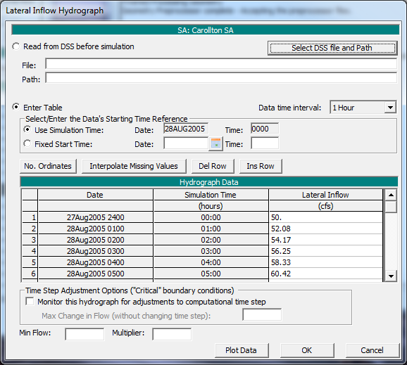

Initial Conditions

Initial conditions consist of flow information at each of the cross sections, as well as elevations for any storage areas defined in the system. Data for initial conditions is established by selecting the Initial Conditions tab on the Unsteady Flow Data Editor. After selecting the tab, the figure below will be displayed.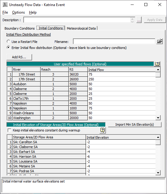As seen in the figure above, the Enter Initial flow distribution radio button was selected and initial flows were entered at the upstream river station of each of the 11 reaches. The initial elevation of all eight storage areas was set to the minimum storage area elevation by clicking Import Min SA Elevation(s). The Initial Elevation field is then populated with all the storage area's minimum elevation from the Geometric Editor. The data was then saved (File -> Save Unsteady Flow Data As) in the Unsteady Flow Data Editor and the window was closed.

Unsteady Flow Analysis

After the geometry and unsteady flow data have been completed an unsteady flow analysis may be initiated. Under the main program window Unsteady Flow Analysis was selected under the Run menu. This will display the Unsteady Flow Analysis Window shown below.  A plan was defined by selecting the Geometry File "Orleans Parish – Existing Conditions" and the Unsteady Flow File "Katrina Event." Under the File menu, Save Plan As was selected and the plan title was entered as "Katrina Existing Conditions." After entering the title of the plan a short identifier was entered as "KatrinatExist" and the plan was saved. The data was entered as seen in the figure below. For more information on the Simulation Time Window, Computation Settings, and Programs to Run refer to Unsteady Flow Application – Example 17.

Note: The data entered for the levee breach in the Geometric Data Editor can also be entered through the Unsteady Flow Analysis window. The user can open the Levee (Lateral Structure) Breach Data by clicking on Options then Levee (Lateral Structure) Breach from the Unsteady Flow Analysis window.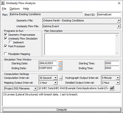

Output Analysis

For the analysis of the output, a portion of the system's Water Surface Profiles were reviewed, as well as the Stage and Flow Hydrographs for the pump station. These are discussed in the following sections.

Water Surface Profiles

The water surface profiles are shown in the figure below by selecting View and then Water Surface Profiles. The figure shows the maximum water surface profile on Reach 1 and 2 of both 17^th Street and Claiborne. The lighter gray structures represent lateral structures, whereas the darker gray area represents a cross section lid. From the figure below it can be seen that the water surface elevation rises above the bottom of the lid and is identical to the energy grade line. The water surface profile is actually a representation of the water surface within a very small opening that extends through the top of the lid. This small opening is necessary for using the Priessmann slot theory, which is the method that allows pressurized pipes to be modeled with unsteady flow in HEC-RAS.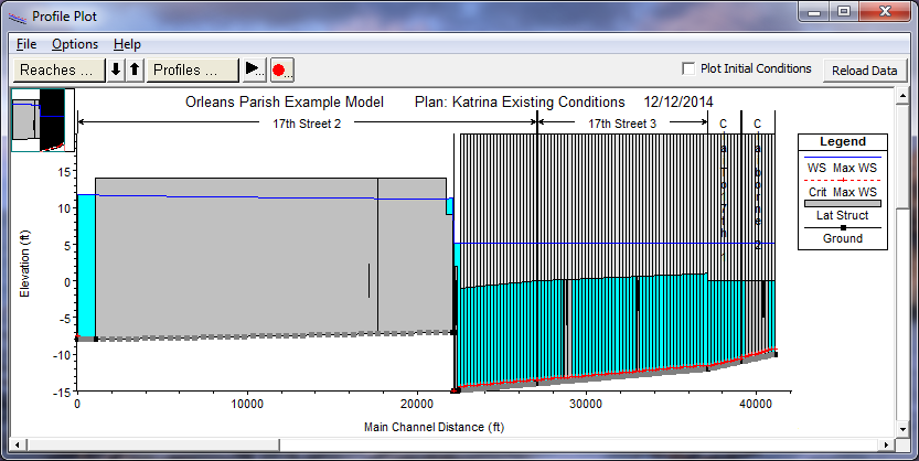

Stage and Flow Hydrographs

The output from the simulation can be viewed from many different tables and graphs. The most interesting output for the pump station in this example is found by viewing the stage and flow hydrographs. From the main program window, View and then Stage and Flow Hydrograph was selected. By selecting the Type menu on the Stage and Flow Hydrograph Window the user can view stage and flow hydrographs for cross sections, bridges, culverts, inline structures, lateral structures, storage areas, storage area connections, and pump stations.

The "Pump Stations" option was selected from the Type menu, which then displayed the stage and flow hydrographs seen in the figure below. As seen from the figure, the initial headwater stage was -4 feet. Therefore, only one pump was turned on (see Pump Station Data Editor), producing a flow of approximately 200 cfs. At 10 A.M. on August 28 the flow abruptly increased to approximately 400 cfs, followed by a stint with a steady pump rate around 400 cfs, and then a drop in flow back to approximately 200 cfs. This process was repeated and at 12 P.M. on August 29 the pump rate went to 100 and remained there for the remainder of the simulation. This can be explained by simultaneously reviewing the hydrographs with the pump station data. The increases in pump rate are due to the increase in the headwater stage from -4 feet to -3 feet. According to the pump data, this increase caused another pump to turn on, thereby increasing total flow by nearly 200 cfs. The increased pumping rate subsequently caused the headwater stage to decrease, thereby turning off one of the pumps and reducing the pump rate. This process was repeated until at 12 P.M. on August 29 the Advanced Control Rules from the Pump Station Data Editor was activated. The rule caused all subsequent flow rates from the pump station to hold steady at 100 cfs.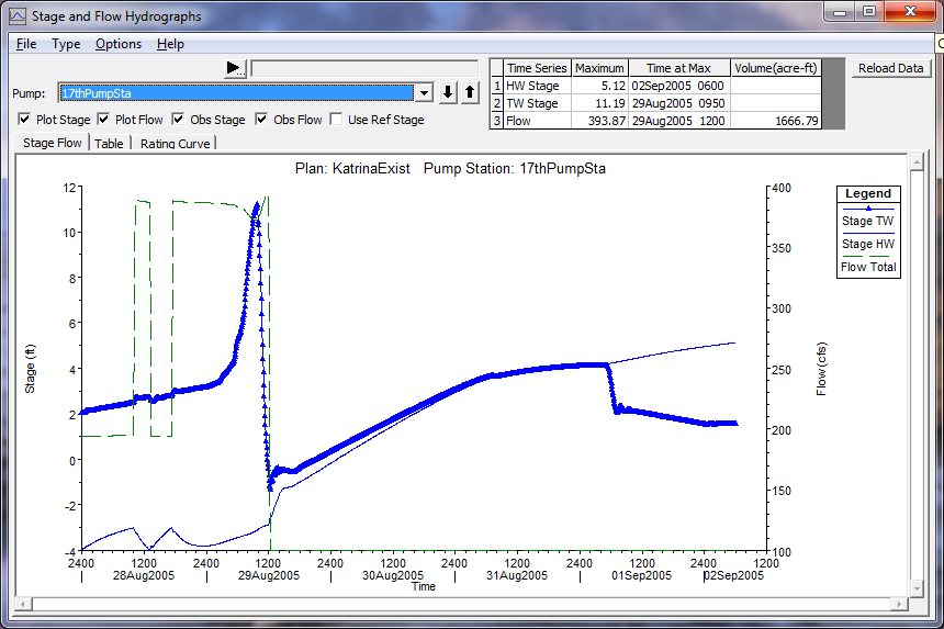

Summary

Urban modeling is unique in that it often incorporates several HEC-RAS elements that many river systems don't utilize. This example gave note to many of those features - pressurized pipe flow, how to model pipe connections, drop inlets, minor losses, levee breaches, interconnected storage areas (surface overland flow system) and pump stations – by modeling a portion of a New Orleans Parish system. For many of these features, the user was shown how to access them from the Geometric Data Editor. For instance, the user was shown how to turn a typical cross section into a pipe by using the Lid feature which is accessed through the Cross Section Editor. After entering all of the geometric data, the user was shown how to enter the unsteady flow data, as well as the plan information. Once the model was run, some of the relevant output data is reviewed.