The current version of HEC-RAS includes two hydrodynamic approaches to Sediment Transport Analysis:
- Quasi-Unsteady Flow and
- Unsteady Flow.
HEC-RAS allows users to run Quasi-unsteady flow simulations without sediment transport (e.g. for riparian vegetation analysis) but sediment transport models are the most common application of the quasi-unsteady flow method. The quasi-unsteady hydrodynamic model simulates the flow series with a sequence of steady flow computations (the (a) Quasi Unsteady Histograph plots on the left, below). Hydrodynamic parameters for the sediment model are computed with the HEC-RAS steady flow engine, then applied over specified time windows to compute sediment transport temporally.
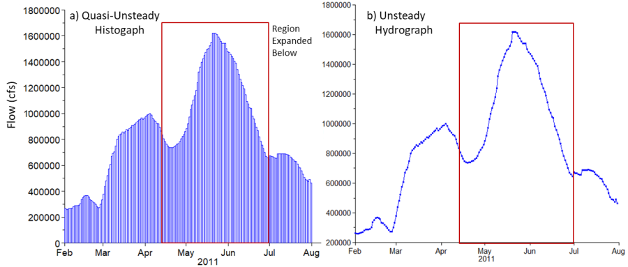
 the quasi-unsteady flow model (a series of steady flows or 'histograph') and (b) the unsteady flow model.")
Unsteady sediment transport capabilities are new in HEC-RAS version 5.0 (The (b) Unsteady Hydrograph plots on the right above). HEC-RAS can run unsteady flow simulations without sediment. Setting up unsteady flow files and troubleshooting unsteady flow models are covered in detail in Chapter 8 (Performing and Unsteady Flow Analysis). Constructing an accurate, calibrated, stable unsteady hydraulic model is the first step in unsteady sediment modeling.
Selecting the appropriate hydrodynamic model for an HEC-RAS sediment transport analysis involves classic trade-offs between precision and effort (Gibson 2013). Quasi-unsteady modeling tends to be easier, but because it does not conserve flow, it can introduce unacceptable errors, particularly in systems with significant storage.
Unsteady flow modeling requires careful and skillful practice because the solution can be unstable with a fixed bed. Moving unsteady model cross sections can make model stability problems worse, because bed change can introduce instabilities. Making an unsteady flow model robust is not trivial. However, unsteady flow conserves mass and accounts explicitly for volume change, making it particularly applicable for reservoir modeling (Gibson and Boyd, 2014), models with lateral structure flows, reverse flows, or engineering problems where hydrograph timing is critical.
The table below summarizes the costs and benefits of the two approaches and the tree diagram above it outlines the file structure of both approaches.
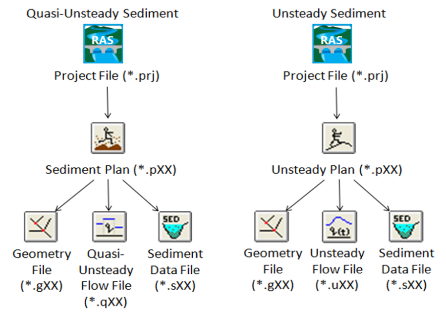
File structure for quasi-unsteady and unsteady sediment transport models.
Table 1 1: Decision Criteria for Selecting Unsteady or Quasi-Unsteady Sediment Simulations.
Quasi-Unsteady | Unsteady |
Solves the steady flow backwater equations for a series of flows with associated times (a histograph). | Solves the Saint-Venant equation implicitly. |
Does not conserve flow or account for storage. | Conserves flow and accounts for reservoir storage. |
More stable. | Less stable. Bed change can exacerbate the unsteady model instabilities, common to the Saint-Venant solution. |
Individual time steps take longer, but the variable time step feature usually translates into shorter model runs. | The unsteady flow engine is faster than steady flow, so each unsteady computation is faster. But the unsteady hydraulics usually require a smaller time step for stability, which makes run times longer.* |
Limited to steady flow options. | Complex flow boundary conditions available including groundwater interflow, rules, lateral structures, internal boundary gate controls, pumps and others. |
*Version 5.0 and later include variable time steps in unsteady simulations and 6.0 decoupled the flow and sediment time steps, giving users some flexibility with these time steps. But unsteady flow runs are still, generally, more computationally expensive.