Sediment Transport Energy Slope

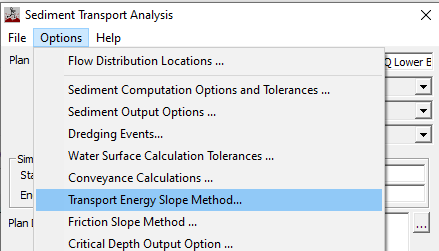
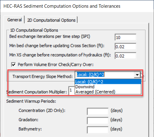
Most sediment transport equations are very sensitive to Slope. These models tend to use the friction slope, which is the slope of the energy grade line. But there are different ways to compute that slope that can generate divergent results under some conditions. You can select the appropriate transport energy slope method under the Sediment Computational Options (Note: this moved to the Computational Options in version 6.3)

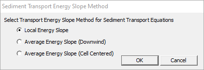
This slope does not affect the hydraulic calculations. HEC-RAS only uses it in the sediment transport equations. The model includes three approaches, illustrated in the following figure and described below.

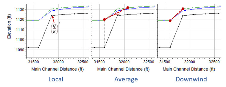
Local Energy Slope Method (Default)

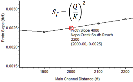
By default HEC-RAS computes this slope locally at the cross section by back calculating the friction slope from Manning's equation (Local Energy Slope), which in US Customary units, is:

$\begin{array}{l}\displaystyle S_f = \left( \frac {Flow}{Conveyance} \right) ^2 = \left( \frac {Flow}{\frac {1.486AR^{\frac23}}{n}} \right) ^2\end{array}$

This is the Friction Slope that HEC-RAS computes and reports in the Hydraulic Results:

However, other models use the slope of the Energy Grade Line across multiple cross sections. This can improve results if the model includes a sharp slope change. These are the Average energy slope methods.

Average Energy Slope - Cell Centered

The Cell Centered Average Energy Slope (Average Energy Slope (Cell Centered)) computes a gradient between the Energy Grade Lines (EGLs - Green Line in Default RAS results) upstream and downstream of the computational cross section:

$\begin{array}{l}\displaystyle S_f = \frac {EGL_{US \space XS} - EGL_{DS\space XS}}{DS \space Dist_{US \space XS} + DS \space Dist_{XS}}\end{array}$

Where:

EGL_{US XS} is the Energy Grade Elevation at the cross section upstream of the computational node,
EGL_{DS XS} is the Energy Grade Elevation at the cross section downstream of the computational node,
DS Dist_{US XS} is the downstream channel distance associated with the cross section upstream of the computational node (distance between the upstream cross section and the computational cross section) and
DS Dist _XS is the downstream channel distance associated with the computational node (distance between the computational cross section and the next cross section downstream).

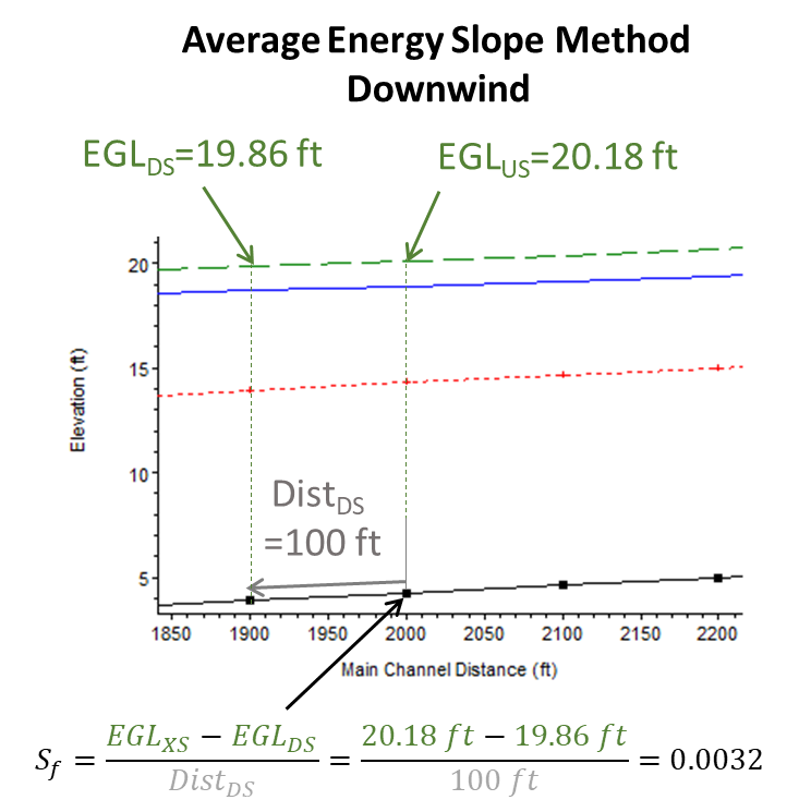
Average Energy Slope - Downwind

Sometimes the Cell Centered Average Energy Slope (Average Energy Slope (Cell Centered)) causes numerical instabilities (leap-frog errors). Therefore, versions 6.2 and later include an alternate form that computes the slope of the energy grade line between the computational cross section and the next cross section downstream (Average Energy Slope (Downwind))

$\begin{array}{l}\displaystyle S_f = \frac {EGL_{XS} - EGL_{DS\space XS}}{DS \space Dist_{XS}}\end{array}$

Where:

EGL_XS is the Energy Grade Elevation at the computational cross section,
EGL_{DS XS} is the Energy Grade Elevation at the cross section downstream of the computational node, and
DS Dist _XS is the downstream channel distance associated with the computational node (distance between the computational cross section and the next cross section downstream).

Users choose the alternate methods most often when modeling headcuts or dam removals.

New Location in Version 6.3+

This feature moved to make it more promient in version 6.3. In previous versions it had its own menu under the Sediment Analysis Options. It moved to the Computational Options with other modeler decisions.

2D Sediment Workshop Videos
HEC hosted a 2D sediment workshop for several district and USACE laboratory modelers using these new tools. Edited videos of most of these talks are included on the HEC training page.