Overview of the Sediment Results Viewer

Tabular Results in 6.5

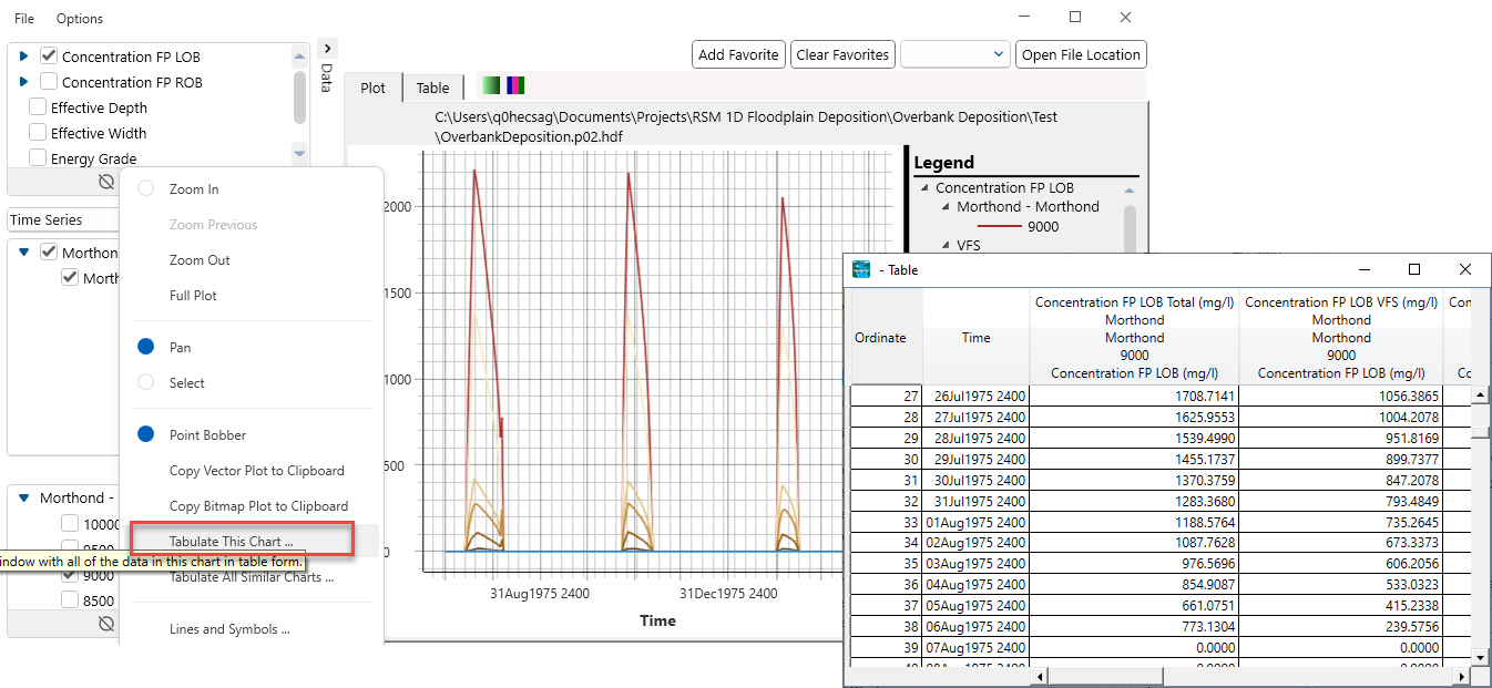
Note: There is a bug in version 6.5 that fails to write the tabular results to the "Table" in the sediment plotter.

Fortunately there is an easy work around for this.  Right click on the plot and select the option to Tabulate this Chart... will launch a new table with the data plotted.

The sediment results viewer combines the advantages of the previous viewers and includes several new features. This new viewer allows users to view results from multiple sediment plans at the same time and view simultaneous time series results on separate axes – if they plot meaningfully on different scales.
The new sediment results viewer has the same three modes that previous viewers had.

• Time Series
• Profile
• Cross section

There is no button on the main HEC-RAS editor to view sediment results. To access Sediment Results Select *ViewSediment Output (6.0)…* from the main HEC-RAS menu (see figure below).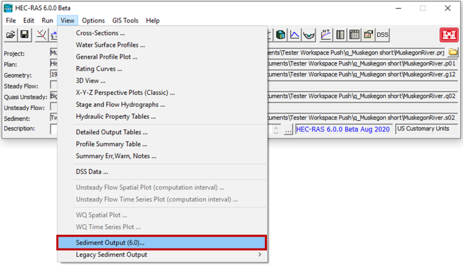

Time Series

Time series results can be extremely valuable to analyze after a sediment transport simulation. To view sediment time series select the Time Series mode on the left bar of the Sediment Results Viewer. Then select one or more variables to plot in the upper left box and one or more cross sections to view them in the lower left box. The first figure below plots regular month-averaged temperature the model used and several years of concentration results for a single cross section. These results plot on separate axes (concentration left, temperature right) because they report in different magnitudes. The color scheme and line weights were edited (right click on plot and select Lines and Symbols to edit lines or add points). To get tabular data click on the Table tab.

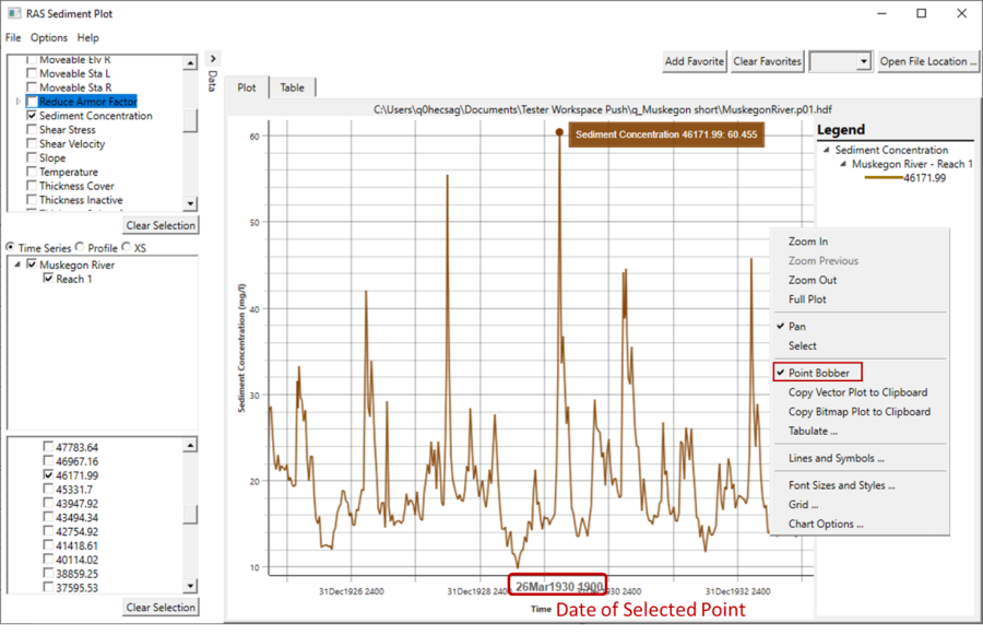
The second plot below demonstrates how to query the value and date of individual points from a time series plot. Right click on the plot and turn on the Point Bobber. Once the Point Bobber is on, you can hover over a location on the time series (like the peak concentration in the figure below) and the plotter will return the value and provide the date and time of the value along the time axis.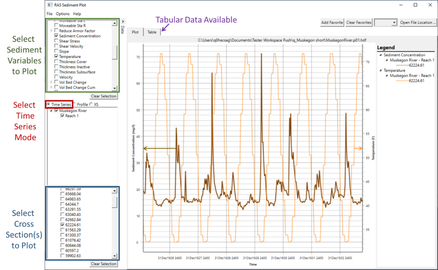

Profile

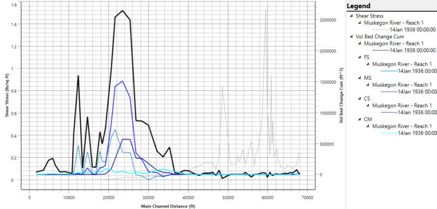
Profiles can be useful for several analyses, but they are used most often to evaluate bed change and bed gradation evolution. The figure below plots Longitudinal Cumulative Volume Change for a reservoir model (positive slope is deposition the downstream value is the total net bed change for the simulation) with several of the most important grain classes and shear stress (light grey). The results show the river deposits in the low shear backwater, and the grain classes deposit in different locations. The second plot shows the same results, but with the cumulative volume change (total for the simulation but not summed from upstream to downstream).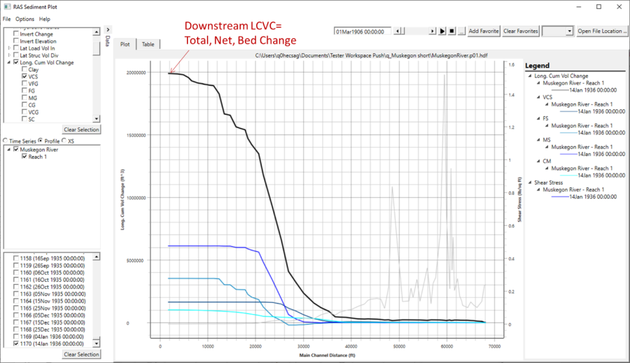

Modeling Note: Expect a Time Lag the First Time the Plotter Accesses Profile Data

The HEC-RAS data model makes retrieving time series data much faster than retrieving profile data. Therefore, profile data can lag more than time series data in the sediment viewer. This should only happen the first time you request a particular profile variable. HEC-RAS will generate a sub-folder with a transposed results file, that the plotter can access more efficiently if the modeler requests the profile data again.

Cross Sections

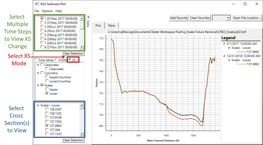
Cross section change is one of the central features of a mobile boundary sediment transport model. Reviewing cross section change is also one of the easiest way to identify numerical artifacts and unintended consequences of modeling choices, making models more realistic and robust. To view cross section change select XS button in the left pane of the Sediment Plotter. The upper pane will populate the time stamps that HEC-RAS generated cross section output and the lower left pane lists the cross sections available to view. Plot the cross sections at multiple time steps to help visualize cross section change. It is important to view at least the final cross section shapes to make sure that erosion and deposition were simulated in physically believable patterns.

Modeling Note: Station Elevation Points

The sediment results viewer only includes lines (no points) by default. Points take require more resources to render, slowing the plotter down substantially. But station-elevation points are often helpful when viewing cross section results. To turn points on, right click on the results, and select Lines and Symbols (see figure below).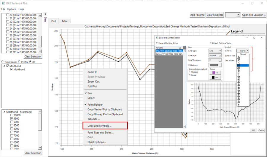

Modeling Note: Invert Change Limitation

This can return good results and is appropriate for scour chains but can also lead to data distortions and does not optimize the value of repeated cross sections or bathymetry data. Computing mass or volume change from repeated cross sections or bathymetry and comparing to Mass/Vol Bed Change CUM or Longitudinal Mass/Vol Change is better modeling practice. (Units: ft or m).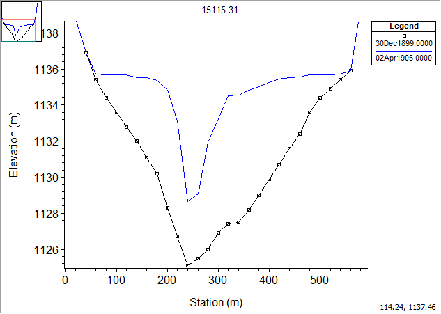

Using Stepped Interpolation to View Quasi-Unsteady Results

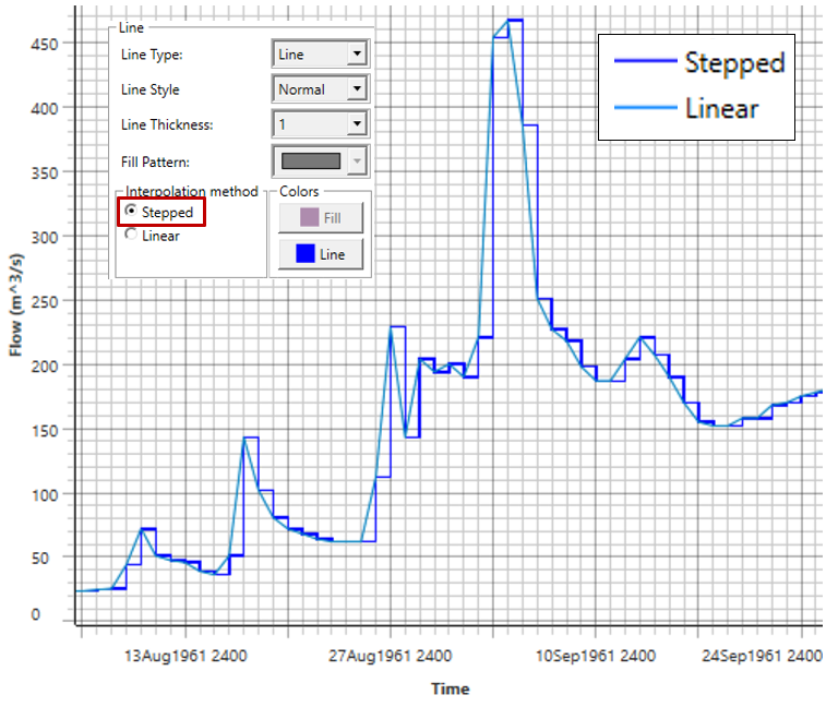
The sediment results viewer has two interpolation approaches.  The default Linear approach draws a straight line between the plotted value at the beginning of the time steps.  Stepped "interpolation," does not interpolate.  The Stepped feature holds the result value constant over the entire time step that it represents.  

Most hydrologic and hydraulic time series in HEC-RAS interpolate.  However, Quasi-Unsteady flow is a series of steady flows.  So the Stepped result can sometimes reflect or report quasi-unsteady results in helpful ways.

Wish List

Plot Water Surface and Movable Bed Limits with Cross Section Results

Wish List

We would like to provide several additional sediment results

• Standard Rating Curves
• User Defined Result Rating Curves (variable 1 vs variable 2, variable 3)
• Sediment gradation curves (particle size vs % finer)
• Gradation over space and time (temporal or longitudinal area plot of grain class %)
• Heat map in time-cross section space (where result magnitude is represented by the color intensity in a time-space plot)
• Specific gage output (plot the water surface elevations associated with defined flow ranges over time)

Wish List

Integrate sediment results into standard HEC-RAS viewers (Rating Curve, generalized profile, hydrograph, etc…)