Download PDF
Download page Cross Section Interpolation.
Cross Section Interpolation
Occasionally it is necessary to supplement surveyed cross section data by interpolating cross sections in between two surveyed sections. Interpolated cross sections are often required when the change in velocity head is too large to accurately determine the energy gradient. An adequate depiction of the change in energy gradient is necessary to accurately model friction losses as well as contraction and expansion losses.
Cross section interpolation can be accomplished in three ways from within the HEC-RAS interface. The first method is to simply copy one of the bounding cross sections and then adjust the station and elevation data. The cross section editor allows the user to raise or lower elevations and to shrink or expand various portions of any cross section. The second and third options allow for automatic interpolation of cross section data. From the Geometric Data editor, automatic interpolation options are found under the Tools menu bar as shown in Figure 5-61.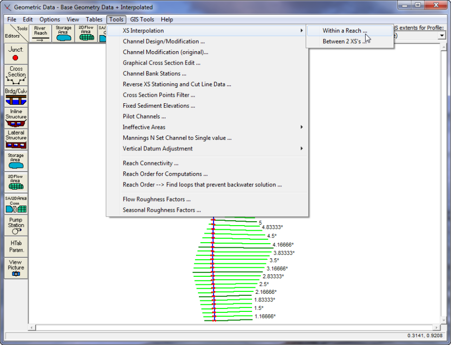
Figure 5 61 Automatic Cross Section Interpolation Options
The first cross section interpolation option, Within a Reach, allows for automatic interpolation over a specified range of cross sections within a single reach. When this option is selected, a window will pop up as shown in Figure 5-62. The user must first select the River and Reach that they would like to perform the interpolation in. Next the user must select a starting River Station and an ending River Station for which interpolation will be performed. The user must also provide the maximum allowable distance between cross sections. If the main channel distance between two sections is greater than the user defined maximum allowable, then the program will interpolate cross sections between these two sections. The program will interpolate as many cross sections as necessary in order to get the distance between cross sections below the maximum allowable. Additionally the user can specify the number of decimal places used for the stationing and elevations of the interpolated cross sections.
Cut Line GIS Coordinates. When cross sections are interpolated, there location on the river system schematic is also interpolated. HEC-RAS has two options for interpolating the coordinates of the cross section cut lines: Linear Interpolation cut lines from the bounding XS's and Generate for display as perpendicular segments to reach invert. The default method is linear interpolation from the bounding cross sections. This method simply draws straight lines between the two cross sections and interpolates the cross section coordinates based on main channel distance. The second method (perpendicular segments to the reach invert line) scales the cross sections along the river reach invert line. A perpendicular segment across the river reach is drawn for the main channel. However, the overbanks are based on average slopes of the invert line upstream and downstream from the point of intersection. 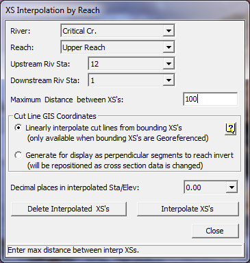
Figure 5 62 Automatic Cross Section Interpolating Within a Reach
Once the user has selected the cross section range and entered the maximum allowable distance, cross section interpolation is performed by pressing the Interpolate XS's button. When the program has finished interpolating the cross sections, the user can close the window by pressing the Close button. Once this window is closed, the interpolated cross sections will show up on the river schematic as light green lines. The lighter color is used to distinguish interpolated cross sections from user-entered data. Interpolated cross sections can be plotted and edited like any other cross section. The only difference between interpolated sections and user-defined sections is that interpolated sections will have an asterisk ![]() attached to the end of their river station identifier. This asterisk will show up on all input and output forms, enabling the user to easily recognize which cross sections are interpolated and which are user defined.
attached to the end of their river station identifier. This asterisk will show up on all input and output forms, enabling the user to easily recognize which cross sections are interpolated and which are user defined.
The second type of automatic cross section interpolation, Between 2 XS's, allows the user to have much greater control over how the interpolation is performed. When this option is selected, a Cross Section Interpolation window will appear as shown in Figure 5-63.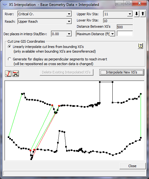
Figure 5 63 Detailed Cross Section Interpolation Window
This cross section interpolation window displays only two cross sections at a time. The user can get to any two cross sections from the River, Reach and River Station boxes at the top of the window. Interpolated cross section geometry is based on a string model as graphically depicted in Figure 561. The string model consists of chords that connect the coordinates of the upstream and downstream cross sections. The cords are classified as master and minor cords. As shown in Figure 5-63, five master cords are automatically attached between the two cross sections. These master cords are attached at the ends of the cross sections, the main channel bank stations, and the main channel inverts. Minor cords are generated automatically by the interpolation routines. A minor cord is generated by taking an existing coordinate in either the upstream or downstream section and establishing a corresponding coordinate at the opposite cross section by either matching an existing coordinate or interpolating one. The station value at the opposite cross section is determined by computing the decimal percent that the known coordinate represents of the distance between master cords and then applying that percentage to the opposite cross section master cords. The number of minor cords will be equal to the sum of all the coordinates of the upstream and downstream sections minus the number of master cords. Interpolation at any point in between the two sections is then based on linear interpolation of the elevations at the ends of the master and minor cords. Interpolated cross sections will have station and elevation points equal to the number of major and minor cords.
This interpolation scheme is used in both of the automated interpolation options ("Within a Reach" and "Between 2 XS's"). The difference is that the Between 2 XS's option allows the user to define additional master cords. This can provide for a better interpolation, especially when the default of five major cords produces an inadequate interpolation. An example of an inadequate interpolation when using the default cords is shown below.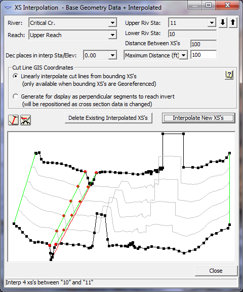
Figure 5 64 Cross Section Interpolation Based on Default Master Cords
As shown in Figure 5-64, the interpolation was adequate for the main channel and the left overbank area. The interpolation in the right overbank area failed to connect two geometric features that could be representing a levee or some other type of high ground. If it is known that these two areas of high ground should be connected, then the interpolation between these two sections should be deleted, and additional master cords can be added to connect the two features. To delete the interpolated sections, press the Del Interp button.
Master cords are added by pressing the Master Cord button that is located to the right of the Maximum Distance field above the graphic. Once this button is pressed, any number of master cords can be drawn in. Master cords are drawn by placing the mouse pointer over the desired location (on the upper cross section), then while holding the left mouse button down, drag the mouse pointer to the desired location of the lower cross section. When the left mouse button is released, a cord is automatically attached to the closest point near the pointer. An example of how to connect master cords is shown in Figure 5-65.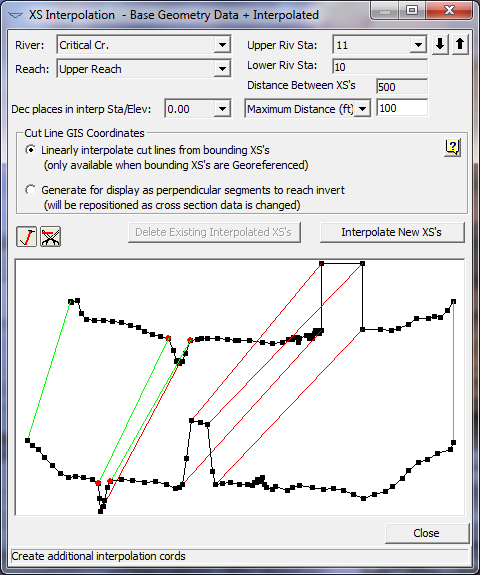
Figure 5 65 Adding Additional Master Cords for Interpolation
User defined master cords can also be deleted. To delete user defined master cords, press the scissors button to the right of the master cords button. When this button is pressed, simply move the mouse pointer over a user defined cord and click the left mouse button to delete the cord.
Once you have drawn in all the master cords that you feel are required, and entered the maximum distance desired between sections, press the interpolate button. When the interpolation has finished, the interpolated cross sections will automatically be drawn onto the graphic for visual inspection. An example of this is shown in Figure 5-66.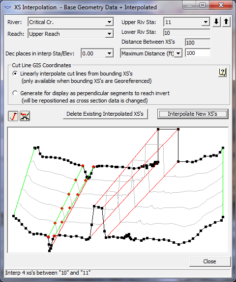
Figure 5 66 Final Interpolation with Additional Master Cords
As shown in Figure 5-66, the interpolation with the addition of user defined master cords is very reasonable.
In general, the best approach for cross section interpolation is to first interpolate sections using the "Within a Reach" method. This provides for fast interpolation at all locations within a reach. The "Within a Reach" method uses the five default master cords, and is usually very reasonable for most cross sections. Once this is accomplished, all of the interpolated sections should be viewed to ensure that a reasonable interpolation was accomplished in between each of the cross sections. This can be done from the "Between 2 XS's" window. Whenever the user finds interpolated cross sections that are not adequate, they should be deleted. A new set of interpolated cross sections can be developed by adding additional master cords. This will improve the interpolation.
An additional option available in the "Between Two XS's" interpolation method is the ability to specify a constant distance for interpolation and to specify a specific location to interpolate a cross section. The Constant Distance option allows the user to put in a distance. This distance will be used to interpolate cross sections starting from the upstream cross section and moving downstream. Once the user entered distance can no longer be met between the two cross sections, then interpolation stops. The second option, Set Location (ft), allows for the interpolation of a single cross section at a specified distance from the upstream cross section.
CAUTION: Automatic geometric cross section interpolation should not be used as a replacement for required cross section data. If water surface profile information is required at a specific location, surveyed cross section data should be provided at that location. It is very easy to use the automatic cross section interpolation to generate cross sections. But if these cross sections are not an adequate depiction of the actual geometry, you may be introducing error into the calculation of the water surface profile. Whenever possible, use topographic maps to assist you in evaluating whether or not the interpolated cross sections are adequate. Also, once the cross sections are interpolated, they can be modified just like any other cross section.
If the geometry between two surveyed cross sections does not change linearly, then the interpolated cross sections will not adequately depict what is in the field. When this occurs, the modeler should either get additional surveyed cross sections, or adjust the interpolated sections to better depict the information from the topographic map.