Download PDF
Download page Steady Flow Data Options.
Steady Flow Data Options
Several options are available from the steady flow data editor to assist users in entering the data. These features can be found under the Options menu at the top of the window. The following options are available:
Undo Editing. This option allows the user to retrieve the data back to the form that it was in the last time the Apply Data button was pressed. Each time the Apply Data button is pressed, the Undo Editing feature is reset to the current information.
Copy Table to Clipboard (with headers). This option allows the user to copy all of the reach, river, river station, and corresponding flow data to the clipboard. This can be very useful if you want to manipulate the data outside of HEC-RAS, such as in Excel.
Delete Row From Table. This option allows the user to delete a row from the flow data table. To use this option, first select the row to be deleted with the mouse pointer. Then select Delete Row From Table from the options menu. The row will be deleted and all rows below it will move up one.
Delete All Rows From Table. This option allows the user to delete all of the rows from the table. To use this option, select Delete All Rows From Table from the Options menu. When this option is selected a window will appear with a question to make sure that deleting all of the row is what you really want to do.
Delete Column (Profile) From Table. This option allows the user to delete a specific column (profile) of data from the table. To use this option, first select the column that you want to delete by placing the mouse over any cell of that column and clicking the left mouse button. Then select Delete Column (Profile) From Table from the Options menus. The desired column will then be deleted.
Ratio Selected Flows. This option allows the user to multiply selected values in the table by a factor. Using the mouse pointer, hold down the left mouse button and highlight the cells that you would like to change by a factor. Next, select Ratio Selected Flows from the options menu. A pop up window will appear allowing you to enter a factor to multiply the flows by. Once you press the OK button, the highlighted cells will be updated with the new values.
Edit Profile Names. This option allows the user to change the profile names from the defaults of PF#1, PF#2, etc.
Set Changes in WS and EG. This option allows the user to set specific changes in the water surface and energy between any two cross sections in the model. The changes in water surface and energy can be set for a specific profile in a multiple profile model. When this option is selected, a window will appear as shown in Figure 6-3. As shown, there are five options that the user can select from: Additional EG, Change in EG, Known WS, Change in WS, and K Loss. The Additional EG option allows the user to add an additional energy loss between two cross sections. This energy loss will be used in the energy balance equation in addition to the normal friction and contraction and expansion losses. The Change in EG option allows the user to set a specific amount of energy loss between two cross sections. When this option is selected, the program does not perform an energy balance, it simply adds the specified energy loss to the energy of the downstream section and computes a corresponding water surface. The Known WS option allows the user to set a water surface at a specific cross section for a specific profile. During the computations, the program will not compute a water surface elevation for any cross section where a known water surface elevation has been entered. The program will use the known water surface elevation and then move to the next section. The Change in WS option allows the user to force a specific change in the water surface elevation between two cross sections. When this option is selected, the program adds the user specified change in water surface to the downstream cross section, and then calculates a corresponding energy to match the new water surface. The K Loss option allows the user to calculate an additional energy loss that will be added into the solution of the energy balance. This energy loss is calculated by taking the user entered K coefficient, times the velocity head at the current cross section being solved. The user entered K coefficient can range from 0.0 to 1.0. The K value is very analogous to a minor loss coefficient, as found in pipe flow hydraulics.
Figure 6 3 Setting Changes in Water Surface and Energy
As shown in Figure 6-3, to use the "Set Internal Changes in WS and EG" option, the user first selects the river, reach, river station, and profile that they would like to add an internal change too. Once the user has established a location and profile, the next step is to select one of the five available options by pressing the appropriate button. Once one of the five buttons are pressed, a row will be added to the table at the bottom, and the user can then enter a number in the value column, which represents the magnitude of the internal change or required coefficient.
Observed WS. This option allows the user to enter observed water surfaces at any cross section for any of the computed profiles. The observed water surfaces can be displayed on the profile plots, cross section plots, and in the summary output tables. To use this option select Observed WS from the Options menu.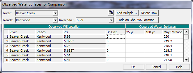
6 4. Observed Water Surface Editor for Steady Flow Analyses.
As shown in Figure 6-4, the user selected a River, Reach, and River Station location, then press the Add an Obs. WS Location (or Add Multiple) to enter a row in the table. Then enter the observed water surface for any of the profiles that are applicable. The column in the table labeled Dn Dist can be used to enter a distance downstream from the currently selected cross section, to further define the actual location of the observed water surface data.
Observed Rating Curves (Gages). This option allows the user to enter an observed rating curve at a gaged location for comparison with computed results. When the user enters an observed rating curve it will show up on the Rating Curve output plot along with the computed water surface versus flow information. To use this option select Observed Rating Curves (Gages) from the Options menu.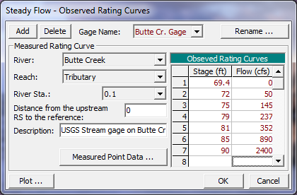
6 5. Observed Rating Curve Editor
As shown in Figure 6-5, the user can Add or Delete a rating curve by pressing one of the buttons at the top. For each rating curve the user is required to select the River, Reach, and River Station that corresponds to the location of the gage. If the gage is not located exactly at one of the user entered cross sections, select the cross section up stream of the gage and then enter a distance downstream from that section to the gage. A description can optionally be entered for the gage. Stage and flow values should be entered for the mean value rating curve at that gage location. In addition to the mean rating curve, the user can enter the actual measured points that went into developing the rating curve. This is accomplished by pressing the Measured Point Data button, which will pop up another editor. In the measured point data editor the user can enter the flow and stage for each measured point that has been surveyed for the gage. Additionally a description can be added for each point (i.e. 72 flood, slope-area measurement, etc…). If measured point data are also entered, then that data will show up on the rating curve plot when comparing the computed water surfaces to the observed.
Gate Openings. This option allows the user to control gate openings for any inline or lateral gated spillways that have been added to the geometric data. When this option is selected, a window will appear as shown in Figure 6-6.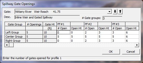
Figure 6 6 Inline Spillway Gated Openings Editor
As shown in Figure 6-6, for each profile the user can specify how many gates are opened per gate group, and at what elevation they are opened too. For the example shown in 6, there are three gate groups labeled "Left Group," "Center Group," and "Right Group." Each gate group has five identical gate openings. All of the gate openings have a maximum opening height of ten feet. For profile number 1, only the middle gate group is opened, with all five gates opened to a height of five feet. For the second profile, all three gate groups are opened. The Left gate group has two gates opened to seven feet, the Center gate group has five gates opened to four feet, and the Right gate group has two gates opened for seven feet. This type of information must be entered for all of the profiles being computed.
Optimize Gate Openings. This option allows the user to have the program compute a gate setting at a structure in order to obtain a user specified water surface upstream of the structure. Given a user entered flow and upstream stage for each profile, the program will iterate with different gate settings until the desired upstream water surface is obtained. This option is very handy when modeling dams and reservoirs.
Initial Split Flow Optimizations (LS and Pumps). This option allows the user to enter initial estimates of the flow that is leaving the main river through a lateral structure or a pump station. Flow values can be entered for each profile. When a value is entered for this option, that amount of flow is subtracted from the main river before the first profile is computed. This option can be useful in reducing the required computation time, or allowing the program to reach a solution that may not otherwise been obtainable.
Inline and Lateral Structure Outlet TS Flows: There is an option on the Inline Structure editor to add a time series of flows type of outlet. This is generally used for Unsteady flow modeling and representing hydropower flows. However, if you are running a model in Steady Flow mode, you can still use this feature. The flow data for this feature will be just the flow rate for this outlet for each profile. The flow entered is a portion of the total flow going through the inline structure for that specific profile.
Storage Area Elevations. This option allows the user to enter water surface elevations for storage areas that have been entered into the geometric data. Storage areas are most often used in unsteady flow modeling, but they may also be part of a steady flow model. When using storage areas within a steady flow analysis, the user is required to enter a water surface elevation for each storage area, for each profile.