Download PDF
Download page Simulation Options.
Simulation Options
The following is a list of the available simulation options under the Options menu of the Steady Flow Analysis window:
Encroachments. This option allows the user to perform a floodway encroachment analysis. For a detailed description of how to use the floodway encroachment capabilities of HEC-RAS, see Chapter 9 of the User's Manual (this manual). For a description of how the encroachment calculations are performed for the various encroachment methods, see Chapter 9 of the Hydraulic Reference Manual.
Flow Distribution Locations. This option allows the user to specify locations in which they would like the program to calculate flow distribution output. The flow distribution option allows the user to subdivide the left overbank, main channel, and right overbank, for the purpose of computing additional hydraulic information.
As shown in Figure 6 10, the user can specify to compute flow distribution information for all the cross sections (this is done by using the Global option) or at specific locations in the model. The number of slices for the flow distribution computations must be defined for the left overbank, main channel, and the right overbank. The user can define up to 45 total slices. Each flow element (left overbank, main channel, and right overbank) must have at least one slice. The flow distribution output will be calculated for all profiles in the plan during the computations.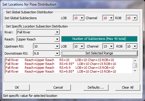
Figure 6 10 Window for Specifying the Locations of Flow Distribution
To set the flow distribution option for all the cross sections, simply select the number of slices for the left overbank, main channel, and right overbank from the Set Global Subsections portion of the window. To set flow distribution output at specific locations, use the Set Specific Location Subsection Distribution option.
During the normal profile computations, at each cross section where flow distribution is requested, the program will calculate the flow, area, wetted perimeter, percentage of conveyance, and average velocity for each of the user defined slices. For details on how the flow distribution output is actually calculated, see Chapter 4 of the HEC-RAS Hydraulic Reference Manual. For information on viewing the flow distribution output, see Chapter 9 of the User's Manual (this manual).
Conveyance Calculations. This option allows the user to tell the program how to calculate conveyance in the overbanks. Two options are available. The first option, At breaks in n values only, instructs the program to sum wetted perimeter and area between breaks in n values, and then to calculate conveyance at these locations. If n varies in the overbank the conveyance values are then summed to get the total overbank conveyance. The second option,
Between every coordinate point (HEC-2 style), calculates wetted perimeter, area, and conveyance between every coordinate point in the overbanks. The conveyance values are then summed to get the total left overbank and right overbank conveyance. These two methods can provide different answers for conveyance, and therefore different computed water surfaces. The At breaks in n values only method is the default.
Friction Slope Methods. This option allows the user to select one of five available friction slope equations, or to allow the program to select the method based on the flow regime and profile type. The five equations are:
- Average Conveyance (Default)
- Average Friction Slope
- Geometric Mean Friction Slope
- Harmonic Mean Friction Slope
- HEC-6 Slope Average Method
Set Calculation Tolerances. This option allows the user to override the default settings for the calculation tolerances. These tolerances are used in the solution of the energy equation. Warning !!! - Increasing the default calculation tolerances could result in computational errors in the water surface profile. The tolerances are as follows:
Water surface calculation tolerance: This tolerance is used to compare against the difference between the computed and assumed water surface elevations. When the difference is less than the tolerance, the program assumes that it has a valid numerical solution. The default value is 0.01.
Critical depth calculation tolerance: This tolerance is used during the critical depth solution algorithm. The default value is 0.01.
Maximum number of iterations: This variable defines the maximum number of iterations that the program will make when attempting to balance a water surface. The default value is 20.
Maximum difference tolerance: This tolerance is used during the balance of the energy equation. As the program attempts to balance the energy equation, the solution with the minimum error (assumed minus computed water surface) is saved. If the program goes to the maximum number of iterations without meeting the specified calculation tolerance, the minimum error solution is checked against the maximum difference tolerance. If the solution at minimum error is less than this value, then the program uses the minimum error solution as the answer, issues a warning statement, and then proceeds with the calculations. If the solution at minimum error is greater than the maximum difference tolerance, then the program issues a warning and defaults the solution to critical depth. The computations then proceed from there. The default value is 0.30.
Flow Tolerance Factor: This factor is only used in the bridge and culvert routines. The factor is used when the program is attempting to balance between weir flow and flow through the structure. The factor is multiplied by the total flow. The resultant is then used as a flow tolerance for the balance of weir flow and flow through the structure. The default value is 0.001
Maximum Iteration in Split Flow: This variable defines the maximum number of iterations that the program will use during the split flow optimization calculations. The default value is 30.
Flow Tolerance Factor in Weir Split Flow: This tolerance is used when running a split flow optimization with a lateral weir/gated spillway. The split flow optimization continues to run until the guess of the lateral flow and the computed value are within a percentage of the total flow. The default value for this is 2 percent (.02).
Maximum Difference in Junction Split Flow: This tolerance is used during a split flow optimization at a stream junction. The program continues to attempt to balance flow splitting from one reach into two until the energy gradelines of the receiving streams are within the specified tolerance. The default value is 0.02.
Each of these variables has an allowable range and a default value. The user is not allowed to enter a value outside of the allowable range.
Critical Depth Output Option. This option allows the user to instruct the computational program to calculate critical depth at all locations.
Critical Depth Computation Method. This option allows the user to select between two methods for calculating critical depth. The default method is the Parabolic Method. This method utilizes a parabolic searching technique to find the minimum specific energy. This method is very fast, but it is only capable of finding a single minimum on the energy curve. A second method, Multiple Critical Depth Search, is capable of finding up to three minimums on the energy curve. If more than one minimum is found the program selects the answer with the lowest energy. Very often the program will find minimum energies at levee breaks and breaks due to ineffective flow settings. When this occurs, the program will not select these answers as valid critical depth solutions, unless there is no other answer available. The Multiple Critical Depth Search routine takes a lot of computation time. Since critical depth is calculated often, using this method will slow down the computations. This method should only be used when you feel the program is finding an incorrect answer for critical depth.
Flow Optimizations. This option allows the user to have the program optimize the split of flow at lateral structures, lateral diversions, stream junctions, and pump stations. When this option is selected, a window will appear as shown in Figure 6-11. As shown in Figure 6-11, there are four tabs to choose from. One tab is for each of the following: Junctions; Lateral Weirs/Diversions; Reach-Storage Areas; and Pump Stations.
When the Lateral Weir/Diversion tab is selected, a table with all of the lateral weirs/spillways and rating curves defined in the model will be displayed. To have the program optimize the split of flow between the main stream and a lateral weir/spillway (or rating curve), the user simply checks the column labeled "Optimize." If you do not want a particular lateral weir/spillway to be optimized, the user should not check the box. For the first iteration of the flow split optimization, the program assumes that zero flow is going out of the lateral structure. Once a profile is computed, the program will then compute flow over the lateral structure. The program then iteratively reduces the flow in the main channel, until a balance is reached between the main river and the lateral structure. The user has the option to enter an initial estimate of the flow going out the lateral structure. This can speed up the computations, and may allow the program to get to a solution that may not have otherwise been possible. This option is available by selecting "Initial Split Flow Values" from the "Options" menu of the Steady Flow Data editor.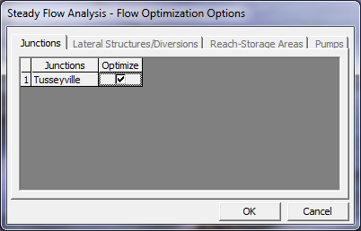
Figure 6 11 Split Flow Optimization Window
When the Junction tab is selected, the table will show all of the junctions in the model that have flow splits. To have the program optimize the split of flow at a junction, check the optimize column, otherwise leave it unchecked. Flow optimizations at junctions are performed by computing the water surface profiles for all of the reaches, then comparing the computed energy grade lines for the cross sections just downstream of the junction. If the energy in all the reaches below a junction is not within a specified tolerance (0.02 feet), then the flow going to each reach is redistributed and the profiles are recalculated. This methodology continues until a balance is reached.
When the Reach – Storage Areas tab is selected, a window will appear displaying all of the storage areas that are upstream boundaries to river reaches. If optimization is set to on for a particular storage area, the program will optimize the amount of flow coming out of the storage area, based on the user specified elevation of the storage area.
The final tab is for Pumps. When this tab is pressed a table will appear showing all of the locations where pump stations are connected to the main rivers. The user can then turn on optimization for the split of flow between the main river and the pump station.
Check Data Before Execution. This option provides for comprehensive data input checking. When this option is turned on, data input checking will be performed when the user presses the compute button. If all of the data are complete, then the program allows the steady flow computations to proceed. If the data are not complete, or some other problem is detected, the program will not perform the steady flow analysis, and a list of all the problems in the data will be displayed on the screen. If this option is turned off, data checking is not performed before the steady flow execution. The default is that the data checking is turned on.
Set Log File Output Level. This option allows the user to set the level of the Log file. The Log file is a file that is created by the computational program. This file contains information tracing the program process. Log levels can range between 0 and 10, with 0 resulting in no Log output and 10 resulting in the maximum Log output. In general, the Log file output level should not be set unless the user gets an error during the computations. If an error occurs in the computations, set the log file level to an appropriate value. Re-run the computations and then review the log output, try to determine why the program got an error.
When the user selects Set Log File Output Level, a window will appear as shown in Figure 6-12. The user can set a "Global Log Level," which will be used for all cross sections and every profile. The user can also set log levels at specific locations for specific profiles. In general, it is better to only set the log level at the locations where problems are occurring in the computations. To set the specific location log level, first select the desired reach and river station. Next select the log level and the profile number (the log level can be turned on for all profiles). Once you have everything set, press the Set button and the log level will show up in the window below. Log levels can be set at several locations individually. Once all of the Log Levels are set, press the OK button to close the window.
View Log File. This option allows the user to view the contents of the log file. The interface uses the Windows Write program to accomplish this. It is up to the user to set an appropriate font in the Write program. If the user sets a font that uses proportional spacing, the information in the log file will not line up correctly. Some fonts that work well are: Line Printer; Courier (8 pt.); and Helvetica (8 pt.). Consult your Windows user's manual for information on how to use the Write program.
View Runtime Messages File. This option will allow the user to open a file that contains the runtime messages from the last time the Steady Flow model was computed.
Figure 6 12 Log File Output Level Window