Download PDF
Download page Mixed Flow Regime.
Mixed Flow Regime
Modeling mixed flow regime (subcritical, supercritical, hydraulic jumps, and draw downs) is quite complex with an unsteady flow model. In general, most unsteady flow solution algorithms become unstable when the flow passes through critical depth. The solution of the unsteady flow equations is accomplished by calculating derivatives (changes in depth and velocity with respect to time and space) in order to solve the equations numerically. When the flow passes through critical depth, the derivatives become very large and begin to cause oscillations in the solution. These oscillations tend to grow larger until the solution goes completely unstable.
In order to solve the stability problem for a mixed flow regime system, Dr. Danny Fread (Fread, 1986) developed a methodology called the "Local Partial Inertia Technique." The LPI method has been adapted to HEC-RAS as an option for solving mixed flow regime problems when using the unsteady flow analysis portion of HEC-RAS. This methodology applies a reduction factor to the two inertia terms in the momentum equation as the Froude number goes towards a user entered Froude Number Threshold (Default = 0.8). The modified momentum equation is show below:
| \sigma \left[\frac{\delta Q}{\delta t} + \frac {\delta \left( \frac{\Beta Q^2}{A }\right)}{\delta x}\right] + g A\left( \frac {\delta h}{\delta x} + S_f \right) |
and
| \sigma = 1.0 - \left( \frac{F_r}{F_T} \right)^m \;\;\;\;\;\;\;\;\;\; (F_r \le F_T ; \;\; m \ge 1) |
| \sigma = 0 \;\;\;\;\;\;\;\;\;\;\;\;\;\;\;\;\;\;\;\;\;\;\;\;\;\;\;\;\;\; (F_r > F_T) |
where:
σ = LPI factor to multiply by inertial terms.
FT = Froude number threshold at which factor is set to zero. This value has a practical application range from 0.0 to 2.0 (default is 0.8). If you use zero, the inertial terms are always zeroed out, and in affect you have a Diffusion Wave routing scheme, rather than Full Unsteady Flow equations.
Fr = Froude number.
m = Exponent of equation, which changes the shape of the curve. This exponent can range between 1 and 128 (default value is 4). A practical upper limit would be 32.
h = Water surface elevation
Sf = Friction slope
Q = Flow rate (discharge)
A = Active cross sectional area
g = Gravitational force
The default values for the equation are FT = 0.8 and m = 4. When the Froude number is greater than the threshold value, the factor is set to zero. The user can change both the Froude number threshold and the exponent. As you increase the value of both the threshold and the exponent, you decrease stability but increase accuracy. As you decrease the value of the threshold and/or the exponent, you increase stability but decrease accuracy. To change either the threshold or the exponent, select 1D Mixed Flow Options tab from the Options/Computational Options and Tolerances menu of the Unsteady Flow Analysis window. When this option is selected, the unsteady mixed flow options window will appear as shown in Figure 14-1.
As shown in Figure 14-1, the graphic displays what the magnitude of the LPI factor will be for a given Froude number and a given exponent m. Each curve on the graph below represents an equation with a threshold of 1.0 (FT) and a different exponent (m).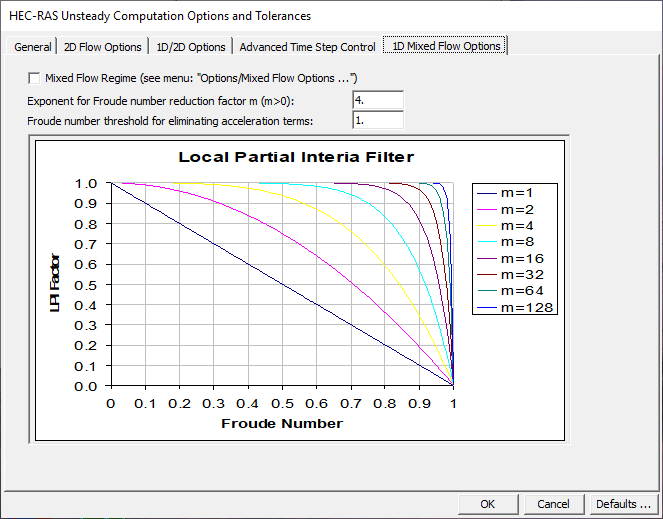
Figure 14 1. Unsteady Mixed Flow Options Window
By default, the mixed flow regime option is not turned on. To turn this option on, check the Mixed Flow Regime box, which is contained at the top of the Mixed Flow regime window. This window and option is shown in the Figure 14-2.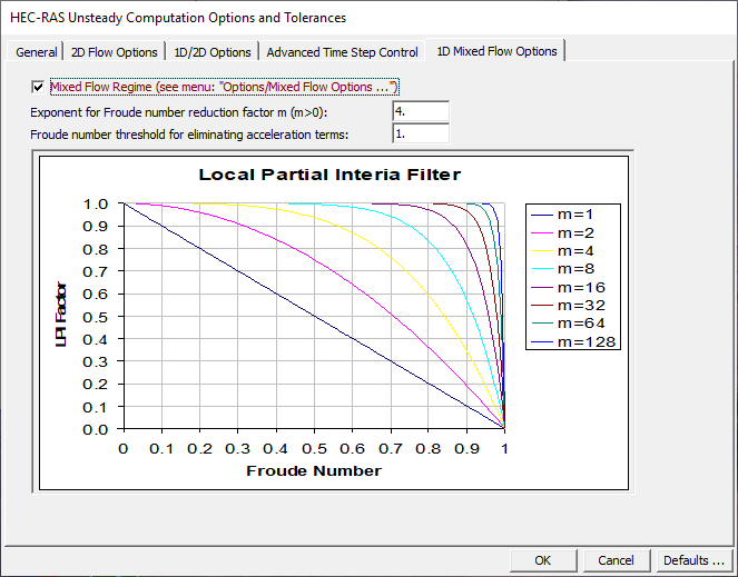
Figure 14 2. Unsteady Flow Analysis Window with Mixed Flow Regime Option Turned On
In general, when modeling a river system that is completely subcritical flow, you should not turn on the mixed flow regime option. If the system is mostly subcritical flow, with only a few areas that pass through critical depth, then this option can be very useful for solving stability problems. However, there may be other options for modeling the areas that pass through critical depth. For example, if the system has a location with a drops in the bed where flow passes through critical depth over the drop, but is subcritical just downstream of the drop, this would be a good location to model the drop as an inline weir within HEC-RAS. By modeling the drop as an inline weir, the program is not modeling the passing through critical depth with the momentum equation, it is getting an upstream head water elevation for a given flow from the weir equation. If the river system has several areas that pass through critical depth, go supercritical, and go through hydraulic jumps, then the mixed flow methodology may be the only way to get the model to solve the unsteady flow problem.
A profile plot of a mixed flow regime problem is shown in Figure 14-3. This example was run with the unsteady flow simulation capability within HEC-RAS using the mixed flow regime option. The example shows a steep reach flowing supercritical, which then transitions into a mild reach. A hydraulic jump occurs on the mild reach. The mild reach then transitions back to a steep reach, such that the flow goes from subcritical to supercritical. Because of a high downstream boundary condition (for example backwater from a lake), the flow then goes from supercritical to subcritical though another hydraulic jump. 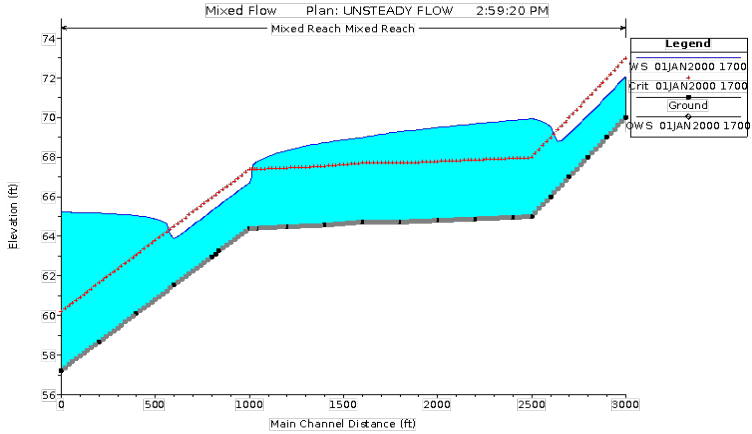
Figure 14 3. Example Mixed Flow Regime Run with Unsteady Flow Routing