Download PDF
Download page Sediment Transport Capacity.
Sediment Transport Capacity
The sediment transport capacity computations can only be run once steady or unsteady flow computations have been run. Sediment Transport Capacity for any cross section can be computed using any of the following sediment transport functions:
- Ackers-White
- Engelund-Hansen
- Laursen
- Meyer-Peter Müller
- Toffaleti
- Yang
To access the sediment transport capacity window, click on Type…Sediment Transport Capacity in the Hydraulic Design Window. The following window will become active: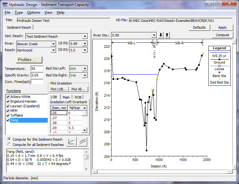
Figure 13 12. Sediment Transport Capacity Window
To perform sediment transport capacity computations, the user must define one or more sediment reaches. A sediment reach indicates for which cross sections transport rates will be computed and contains information necessary to fulfill the computations. Sediment reaches can vary spatially within the geometry, can have different input parameters such as temperature, specific gravity, and gradation, or can simply use different sediment transport functions. A sediment reach cannot span more then one river reach, however there can be multiple sediment reaches within one river reach. Sediment reaches cannot have overlapping cross sections.
When the sediment transport capacity window is opened, if there are not any previously defined sediment reaches defined for the current hd file, the user will be automatically prompted to name a new sediment reach. To create a new reach otherwise, click on File…New Sediment Reach. The user also has the option of copying, deleting, and renaming existing sediment reaches under the File menu option. The name selected for the new sediment reach will appear in the Sed. Reach dropdown box along with all other existing sediment reaches for the particular hydraulic design file.
Once a new sediment reach has been named, the user must define its spatial constraints by selecting the river, reach, and the bounding upstream and downstream river stations. Next, one of the existing profiles must be selected.
Sed.Reach: Indicates which sediment reach is active. This dropdown box lists all existing sediment reaches for the current hydraulic design file.
River: The river where the current sediment reach is located.
Reach: The reach where the current sediment reach is located.
US RS: The upstream bounding river station of the current sediment reach.
DS RS: The downstream bounding river station of the current sediment reach.
Profiles: The profile to be used in the sediment transport computations for the current sediment reach.
River Sta: The river station currently displayed on the plot.
Temperature: Temperature of the water. Default is 55 degrees F or 10 degrees C.
Specific Gravity: Specific gravity of the moveable sediments. Default is 2.65.
Bed Sta Left/Right: The cross section stations that separate the left overbank from the main channel from the right overbank for sediment transport capacity computations. Defaults are the main bank stations. These values can be changed for every cross section within the sediment reach. The selected stations appear on the cross section plot as yellow nodes, and are bracketed by "MB" (mobile bed) location arrows on the top of the plot.
Conc. of Fines (opt): The concentration of fine sediments (wash load) in the current sediment reach. This is an optional value and is used to adjust the transport rate based on Colby's (Colby, 1964) findings regarding the effects of fine sediment and temperature on kinematic viscosity, and consequently particle fall velocity. Values are given in parts sediment per one million parts water, by weight.
Functions: The user can select one or more sediment transport functions from this list box. By clicking the checkbox, a check will appear and RAS will compute for that function. When clicking on the name of the function, a brief description of the function and its applicability will appear in the text box below.
Gradation: This is entered for the left overbank (LOB), main channel (Main) and right overbank (ROB) as defined by the left and right bed stations. The user can enter nothing or up to 50 particle size/percent finer relationships. By right-clicking on one of the tabs, the grid can be expanded for easier viewing. Right-click again to return the grid to its compact display. Typically 5 to 10 gradation points are enough to represent a typical gradation curve. The particle diameter is entered in mm under the column header Diam, mm, and the percent of the representative sediment that is finer than that particle diameter is entered under the column header %Finer. RAS then takes this gradation input to determine the fraction of the sediment that is in each standard grade size class. If a zero percent value and/or a 100% value are not entered by the user, the program will assign zero percent to the next lowest grade class and 100% to the next highest grade class. See the hydraulic reference manual for more detail.
Plot Gradation: This button gives the user a graphical representation of the sediment gradation.
The user has the option to compute sediment transport capacity rates for the currently selected sediment reach (Compute for this Sediment Reach) or for all existing sediment reaches (Compute for all Sediment Reaches) within the currently opened hydraulic design file.
A text box is provided for brief descriptions of selected transport functions. In addition to a summary of the selected function, the range of input parameters, from both field and laboratory measurements, used in the development of the respective function is also provided. Where available, these ranges are taken from those found in the SAM package user's manual (Waterways Experiment Station, 1998) and are based on the developer's stated ranges when presented in their original papers. The ranges provided for Engelund and Hansen are taken from the database (Guy, et al, 1966) primarily used in that function's development.
The following variables are used in the summaries:
- d, overall particle diameter
- dm, median particle diameter
- s, sediment specific gravity
- V, average channel velocity
- D, channel depth
- S, energy gradient
- W, channel width
- T, water temperature
Defaults: The Defaults button will restore all input boxes for the currently selected sediment reach to the default values.
Apply: The Apply button will be enabled any time new input has been added which has not been stored into memory. By clicking on the Apply button, all input for the current sediment reach will be stored to memory.
Compute: The compute button will be enabled once all required input is entered. Pressing the compute button initiates the computations for sediment transport capacity.
Options Menu: The Options Menu drop down list is on the top of the Sediment Transport Capacity form and includes:
Fall Velocity: This option allows the user to select the method of fall velocity computation. If "Default" is selected, the method used in the research and development of the respective function is chosen. Otherwise, any functions used in the computations will use the selected fall velocity method. The three fall velocity methods available are: Toffaleti, Van Rijn, and Rubey.
Depth/Width: This allows the user to select which depth and width parameters to use in the solution of the transport functions. If "Default" is selected, the program will use the depth/width combination used in the research of the selected functions(s). If any of the other depth/width combinations is used, all selected functions will be solved using those specific parameters.
Eff. Depth/Eff. Width: Used in HEC 6, this is the effective depth and effective width. Effective Depth is a weighted average depth and the effective width is calculated from the effective depth to preserve aD2/3 for the cross section:
Hyd. Depth/Top Width: The hydraulic depth is the area of the cross section divided by the top width.
Hyd. Radius/Top Width: The hydraulic radius is the Area divided by the wetted perimeter. Is equivalent to hydraulic depth for relatively wide, shallow streams.
Hiding Factor for Ackers-White: An optional "hiding factor" adjustment is available for the Ackers-White function only. The user can choose whether or not to use this feature. The default is "No."
Compute for Small Grains Outside Applicable Range: By default, RAS will perform calculations for grain sizes which are smaller than the applicable range of a given transport function. By selecting "No", the user can override this and have RAS compute for only the grain sizes within the applicability range of each sediment transport function, as defined in Table 12.7 in the Reference Manual.
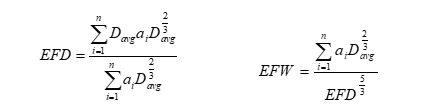
![]() Sediment Rating Curve Plot/Table: This button displays a plot of the sediment transport capacity rates for a selected cross section within a sediment reach. It is only enabled once computations for that reach have been performed. Display options can be selected from the dropdown buttons. Figure 13-13 shows a sediment rating curve plot. In addition to viewing the plots, the table tab can be clicked to view in tabular form.
Sediment Rating Curve Plot/Table: This button displays a plot of the sediment transport capacity rates for a selected cross section within a sediment reach. It is only enabled once computations for that reach have been performed. Display options can be selected from the dropdown buttons. Figure 13-13 shows a sediment rating curve plot. In addition to viewing the plots, the table tab can be clicked to view in tabular form.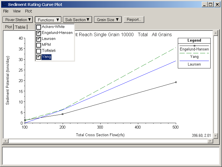
Figure 13 13. Sediment Transport Capacity Rating Curve
![]() Sediment Transport Profile Plot/Table: This button displays a plot of the sediment transport capacity rates along a selected sediment reach. It is only enabled once computations for that reach have been performed. Display options can be selected from the dropdown buttons. Figure 13-14 shows the sediment transport profile plot. In addition to viewing the plots, the table tab can be clicked to view in tabular form.
Sediment Transport Profile Plot/Table: This button displays a plot of the sediment transport capacity rates along a selected sediment reach. It is only enabled once computations for that reach have been performed. Display options can be selected from the dropdown buttons. Figure 13-14 shows the sediment transport profile plot. In addition to viewing the plots, the table tab can be clicked to view in tabular form.
Figure 13 14. Sediment Transport Capacity Plot
Both plot windows have a list box at the bottom with warning messages. These warnings are meant to make the user aware of how sediment transport rates are being computed. If the user selects the option to compute sediment transport rates for all grade sizes within the user-specified range, a warning stating this will be shown. If the user selects the option to compute sediment transport rates for only those grade sizes within the respective function's applicability range, then a warning a different warning message will appear.
The "Compute for Small Grains Outside Applicability Range" option is located in the menu item "Options" on the Hydraulic Design window for sediment transport capacity.
Report: The Report button is located in the plot window and generates a report summarizing the input and output data. The output data is displayed as per the selections made in the dropdown buttons. Because the amount of output has the potential for being quite large, the report that is generated can likewise be very large. Figure 13-15 shows an example of the sediment transport capacity report. As with other report windows found in HEC-RAS, the user has the ability to send this report to the clipboard, print it, or save it as a text file.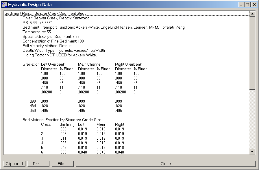
Figure 13 15. Sediment Transport Capacity Report