Download PDF
Download page Developing the River System Schematic.
Developing the River System Schematic
![]()
The modeler develops the geometric data by either first drawing in the river system schematic on the Geometric Data window (Figure 5-1) or by developing a schematic in HEC-RAS Mapper (See the separate HEC-RAS Mapper User's manual). The River System Schematic is a diagram of how the stream system is connected together. The river system is drawn on a reach-by-reach basis, by pressing the River Reach button and then drawing in a reach from upstream to downstream (in the positive flow direction). Each reach is identified with a River Name and a Reach Name. The River Name should be the actual name of the stream, while the reach name is an additional qualifier for each hydraulic reach within that river. A river can be comprised of one or more reaches. Reaches start or end at locations where two or more streams join together or spilt apart. Reaches also start or end at the open ends of the river system being modeled. 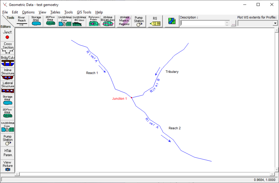
Figure 5 1 Geometric Data Editor Window
Reaches are drawn as multi-segmented lines. Each reach must have at least two points, defining the start and end of the reach. However, it is more typical to draw a reach with several points that would follow along the main channel invert of the stream (this can be accomplished by first loading a background map into the Geometric Data editor). To draw a reach, first press the River Reach button at the top of the Geometric Data editor, on the tools button bar. Move the mouse pointer to the location on the drawing area that you would like to have the reach begin (upstream end of the reach). Click the left mouse button once to define the first point of the reach. Move the mouse and continue to click the left mouse button to add additional points to the reach. To end a reach, move the mouse pointer to the location in which you would like the last point of the reach to be located, then double click the left mouse button. After the reach is drawn, the user is prompted to enter the River Name and the Reach Name to identify the reach. The river and reach identifiers are limited to sixteen characters in length. If a particular River Name has already been entered for a previously defined reach of the same river, the user should simply select that river name from the list of available rivers in the river name text box. As reaches are connected together, Junctions are automatically formed by the interface. The modeler is also prompted to enter a unique identifier for each junction. Junctions are locations where two or more streams join together or split apart. Junction identifiers are also limited to sixteen characters. An example of a simple stream system schematic is shown in Figure 5-1.
In addition to river reaches, the user can draw Storage Areas, 2D Flow Areas, Storage Area/2D Flow Area Connections, Storage Area/2D Flow Area Boundary Condition Lines, and Pump Stations. A storage area is used to define an area in which water can flow into and out of. The water surface in a storage area is assumed to be a level pool. Storage areas can be connected to river reaches as well as other storage areas. The user can connect a storage area directly to the end of a reach or it can be connected to a reach by using the lateral structure option. To connect a storage area to the end of a river reach, simply draw or move the end point of a reach inside of the storage area. Storage areas can be connected to other storage areas hydraulically by using the SA/2D Area Conn option. Storage Area/2D Flow Area connections consist of culverts, gated spillways and a weir. The user can set up a Storage Area/2D Flow Area Connection as just a weir, a weir and culverts, or a weir and gated spillways.
To draw a Storage Area, select the storage area button at the top of the geometric editor window. Storage areas are drawn as polygons. Move the mouse pointer to the location in which you would like to start drawing the storage area. Press the left mouse button one time to start adding points to define the storage area. Continue using single left mouse clicks to define the points of the storage area. To end the storage area, use a double left mouse click. The storage area will automatically be closed into a polygon. Once you have finished drawing the storage area, a window will appear asking you to enter a name for the storage area. To enter and edit the data for a storage area, use the storage area editor button on the left panel of the geometric data window.
To draw a 2D Flow Area, select the 2D Flow Area button at the top of the geometric editor window. 2D Flow areas are drawn as polygons, just like storage areas. Move the mouse pointer to the location in which you would like to start drawing the storage area. Press the left mouse button one time to start adding points to define the storage area. Continue using single left mouse clicks to define the points of the storage area. To end the 2D Flow Area, use a double left mouse click. The 2D Flow Area will automatically be closed into a polygon. Once you have finished drawing the 2D Flow Area, a window will appear asking you to enter a name. To enter and edit the data for a 2D Flow Area, use the 2D Flow Area editor button on the left panel of the geometric data window.
To enter a Storage Area/2D Flow Area Connection, select the SA/2D Area Conn button at the top of the Geometric data editor (this is a hydraulic structure that can be used to connect two storage areas, a storage area to a 2D Flow Area, or two 2D Flow Areas). Move the mouse pointer to the location of left end of the hydraulic structure. SA/2D Area Connections should be drawn from left to right looking in the positive flow direction. Click the left mouse pointer one time to start the drawing of the SA/2D Area Connection. You can continue to use single mouse clicks to add as many points as you want into the line that represents the SA/2D Area Connection. When you want to end the line, double click the mouse pointer. A window will pop up asking you to enter a name for the SA/2D Area Connection. The direction in which you draw the structure is important for establishing the positive flow direction for the flow. If you want the program to output positive flow when the flow is going from one area to another area, then you must draw from left to right looking in the positive flow direction. If flow happens to go in the other direction during the calculations, that flow will be output as negative numbers. To enter and edit the data for a SA/2D Flow Area connection use the SA/2D Area Conn data editor on the left panel of the geometric data window.
To add boundary conditions directly to a 2D Flow Area or a Storage Area, select the SA/2D Area BC Lines button at the top of the Geometric data editor. Move the mouse point to the area of the outer boundary of the 2D Flow Area (or Storage Area) in which you would like to start the boundary condition line. Then click the left mouse pointer one time to start the drawing of the boundary condition line. You can continue to use single mouse clicks, along the outer boundary of the 2D Flow Area, to add as many points as you want into the line that represents the boundary condition. When you want to end the boundary condition line, place the mouse pointer over the location of where you want the line to end, and then double click the mouse pointer. A window will pop up asking you to enter a name for the boundary condition line. These boundary condition lines will show up in the Unsteady Flow Data editor, and will require you to select a boundary condition type (Flow Hydrograph, Rating Curve, or Stage Hydrograph) and enter the necessary data.
Pump stations can be connected between two storage areas, between a storage area and a river reach, or between two river reaches. To add a pump station to the schematic, click the Pump Station button at the top, under the tools button bar, and then left click on the schematic at the location where you want to place the pump station. To connect the pump station, either left click over top of the pump station and select edit, or just click on the pump station editor from the edit tool bar. Connecting pumps is accomplished by picking from and to locations from the pump data editor.
Adding Tributaries into an Existing Reach
If you would like to add a tributary or bifurcation into the middle of an existing reach, this can be accomplished by simply drawing the new reach, and connecting it graphically to the existing reach at the location where you would like the new junction to be formed. This is accomplished by ending the new river reach (tributary) right on top of the location of the main river, where you want the new Junction to be formed. Once the new reach is connected into the middle of an existing reach, you will first be prompted to enter a River and Reach identifier for the new reach. After entering the river and reach identifiers, you will be asked if you want to "Split" the existing reach into two reaches. If you answer "yes", you will be prompted to enter a new Reach identifier for the lower portion of the existing reach (the original reach name is kept for the upper portion of the reach) and a Junction name for the newly formed stream junction.
Editing the Schematic
There are several options available for editing the river system schematic. These options include: changing labels; moving Points/objects (such as labels, junctions, points in a reach or cross section, and 2D area cell centers); adding points (to a reach, cross section, storage area, 2D area boundary, and 2D Flow Area cell centers); deleting points; editing the schematic lines and symbols (line and point types and colors); changing the reach and river station text color; deleting entire reaches, junctions, storage areas/2D Flow Areas, storage area connections, pumps, nodes (cross sections, bridges/culverts, inline structures, lateral structures), and SA/2D Area boundary condition lines. Editing functions for the schematic are found under the Edit menu of the geometric data window. When a specific editing function is selected, the interaction of the user with the schematic is restricted to performing that type of operation. When the user is finished performing that editing function they should turn off that editing function by selecting it again from the Edit menu. When none of the editing functions are turned on, the schematic goes back to the default mode of interaction. The default interaction mode for the schematic is described in the "Interacting with the Schematic" section of this document. A description of each editing function follows:
- Change Name: This option allows the user to change the identifiers of any reach or junction. To change an identifier, you must be in the Change Name edit mode. This is accomplished by selecting the Change Name option from the Edit menu. Once you are in the Change Name edit mode, you then select the particular label that you would like to change by clicking the left mouse button over that label. When a label is selected, a pop up window will appear allowing you to enter a new label. The user can continue to change names by simply selecting the next label to be changed. The Change Name option can only be turned off by re-selecting it from the edit menu or by selecting any other edit option.
- Move Points/Objects: This option allows you to move any label, junction, points in the stream centerline of a reach, points defining the layout of cross sections, storage areas, 2D Flow Area boundaries, and 2D Flow Area cell centers. This is accomplished by first selecting Move Object from the Edit menu, then selecting the particular object that you would like to move. To select an object and then move it, simply place the mouse pointer over the object, then press the left mouse button down. Move the object to the desired location and then release the left mouse button. The Move Object option will remain in effect until the user either turns it off (which is accomplished by re-selecting it) or selects any other edit option.
- Add Points: This option allows the user to add additional points to the line that defines a reach, cross section, storage area, 2D flow area boundaries, and 2D flow Area cell centers. This allows the user to make the schematic be drawn spatially correct as it would be on a map, as well as modify the 2D Flow Area mesh computational cells . To add additional points, first select Add Points from the Edit menu. Move the mouse pointer to the location in which you would like to add an additional point on the reach line, then click the left mouse button. After you have finished adding points to a reach, you can move them around by selecting the Move Object option from the Edit menu. To turn the "Add Points" mode off, simply re-select it from the Edit menu, or select any other edit function.
- Remove Points: This option allows the user to remove points from a reach line, cross section line, storage area, 2D flow area boundary, or 2D Flow Area cell centers. To use this option, first select Remove Points from the Edit menu. Move the mouse pointer over the point that you would like to delete and then click the left mouse button. This option can only be turned off by either re-selecting the option from the Edit menu or by selecting another edit function.
- Lines and Symbols: This option allows the user to change the line and symbol types, colors, and widths for the information on the stream system schematic. When this option is selected a window will appear that shows each line type being used in the schematic. The user can select a particular line type, then change the properties of that line.
- Reach and RS Text Color: This option allows the user to change the color of the text for reaches and river stations plotted on the schematic. The default color is black.
The Edit menu contains an option labeled Delete. The Delete menus has several submenus in order to delete the following objects. - Delete Reach: This option is used to delete a reach. This is accomplished by selecting the Delete Reach option from the Edit menu. A list box containing all the available reaches will appear allowing you to select those reaches that you would like to delete. Warning - Be careful when you delete reaches. When you delete a reach, all of its associated data will be deleted also.
- Delete Junction: This option is used to delete a junction. This is accomplished by selecting the Delete Junction option from the Edit menu. A list box containing all the available junctions will appear allowing you to select those junctions that you would like to delete.
- Delete Storage Areas/2D Flow Areas: This option is used to delete a storage area or a 2D Flow Area. This is accomplished by selecting Delete Storage Areas/2D Flow Areas from the Edit menu. A selection box will appear allowing you to pick the storage areas or 2D Flow Areas that you would like to delete.
- Delete SA/2D Area Connections: This option is used to delete a storage area or a 2D Flow Area hydraulic connection. This is accomplished by selecting the Delete SA/2D Area Connections option from the Edit menu. A list box containing all the available storage area and 2D Flow Area connections will appear allowing you to select the ones that you would like to delete.
- Delete Pump Station: This option allows the user to select one or more pump stations to be deleted from the schematic. This is accomplished by selecting Delete Pump Station from the Edit menu. A list box containing all the available pump stations will appear allowing you to select the ones that you would like to delete.
- Delete Nodes (XS, Bridges, Culverts, etc…): This option allows the user to delete multiple locations at one time. For example, you can delete multiple cross sections at one time with this option. When this option is selected, a window will appear allowing you to select all of the nodes (cross sections, bridges, culverts, Inline structures, lateral structures, etc.) that you would like to delete.
- Delete SA/2D Flow Area Boundary Condition lines: This option is used to delete a storage area or a 2D Flow Area Boundary Condition lines (BC Lines). This is accomplished by selecting the Delete SA/2D Area Boundary Condition lines option from the Edit menu. A list box containing all the available storage area and 2D Flow Area boundary condition lines will appear allowing you to select the ones that you would like to delete.
- Delete 2D Flow Area Breaklines: This option allows the user to delete previously drawn 2D Flow Area Breaklines.
- Delete 2D Flow Manning's Regions: This option allows the user to delete previously drawn 2D Flow Area Manning's n value regions.
Interacting with the Schematic
In addition to modifying the river schematic, there are options available from the View menu to zoom in, zoom previous, zoom out, full plot, pan, set schematic plot extents, and to display or not, many of the river system schematic labels. Additionally, the user has the ability to use the mouse to interact with the schematic. This is accomplished by moving the mouse pointer over an object (river reach line, junction, bridge, culvert, etc…) on the schematic and pressing down the left mouse button. Once the left mouse button is pressed down, a popup menu will appear with options that are specific to that type of object. For example, when the left mouse button is pressed down over a cross section, a menu will appear allowing the user to select options to: edit the cross section, plot the cross section, plot the profile for the reach that the cross section is in, display tabular output for the cross section, and plot the computed rating curve for that cross section.
Another way of interacting with the schematic is to press the right mouse button while the mouse pointer is located anywhere over the schematic drawing area. This will bring up a popup menu that is exactly the same as the View menu at the top of the drawing. This option is providing for convenience in getting to the View menu options.
Cool Graphics Window Tools: Most of the HEC-RAS graphical windows have some cool short cut tools. These tools include the following options:
- Measuring Tool: On any of the graphical windows (Geometric Schematic, Profile Plot, Cross Section Plot, etc…) if you hold down the Cntrl Key, you will get a measuring tool. The measuring tool can be used to draw multi-point lines (polyline) on the graphic window. To draw a polyline, hold down the Cntrl Key and then use single clicks of the left mouse button to start and add points to the line. Double click the left mouse button to end the line. Once you end the line, a window will pop up giving you information about that line, such as: the length of the line; the area if the first and last point were connected to form a polygon; the X-axis length; the Y-axis length; and the slope of the line (dx/dy, from the first point to the last point). Additionally, the X and Y coordinates of the line get sent to the Windows Clipboard, so you can paste those coordinates into a table of some other application. This is a very handy feature for digitizing the coordinates of a cross section, measuring a length, or estimating a slope (i.e. on the profile plot).
- Pan Tool: When you are zoomed in on the graphic within a window, if you hold down the Shift Key, the mouse pointer will change to a hand icon, and you can pan the graphic window. Releasing the Shift Key will change the mouse point back to the original icon.
- Mouse Wheel Feature: Now on any of the HEC-RAS graphical windows, the mouse wheel can be used to Zoom In and Zoom Out. Additionally the graphic will be re-centered based on where the mouse pointer is when using the mouse wheel to zoom in and out.
The following is a list of options available from the View menu:
- Zoom In: This option allows the user to zoom in on a piece of the schematic. This is accomplished by selecting Zoom In from the View menu, then specifying the area to zoom in on with the mouse. Defining the zoom area is accomplished by placing the mouse pointer in the upper left corner of the desired area. Then press down on the left mouse button and drag the mouse to define a box containing the desired zoom area. Finally, release the left mouse button and the viewing area will display the zoomed in schematic. Also displayed will be a small box in the upper right corner of the viewing area. This box will contain a picture of the entire schematic, with a rectangle defining the area that is zoomed in. In addition to showing you where you are at on the schematic, this zoom box allows you to move around the schematic without zooming out and then back in. To move the zoomed viewing area, simply hold down the left mouse button over the rectangle in the zoom box and move it around the schematic. The zoom box can also be resized. Resizing the zoom box is just like resizing a window.
- Zoom Previous: When this option is selected the program will go back to the previously defined viewing window of the schematic. For example, if the user zooms in on the display window of the geometric data editor, then selects the Zoom Previous option, the schematic drawing area will be put back to the previous display area before the last zoom in. The Zoom Previous option will remember up to the last 10 drawing rectangles displayed in the schematic window, so the user can select this option several times in a row to get back to a previous view.
- Zoom Out: This option zooms out to an area that is twice the size of the currently zoomed in window. Zooming out is accomplished by selecting Zoom Out from the View menu on the geometric data window.
- Full Plot: This option re-draws the plot to its full original size. The Full Plot option is accomplished by selecting Full Plot from the View menu on the geometric data window.
- Pan: This option allows the user to move around when in a zoomed in mode. The pan option is accomplished by selecting Pan from the View menu of the geometric data window. When this option is selected, the mouse pointer will turn into a hand. Press the left mouse button and hold it down, then move the mouse. This will allow the user to move the zoomed in graphic. To turn the pan mode off, re-select the pan option from the view menu. A short cut way to use the pan option is to simply hold down the Shift Key while the mouse is over the schematic. This will change the pointer to a hand graphic. Hold down the left mouse button and move the graphic. To stop panning, and change the pointer back to normal, release the Shift key.
- Set Schematic Plot Extents: This option allows the user to set the extents of the viewing area for the river system schematic. The user can enter a specific coordinate system, or utilize the default data system. The default data plot extents are from 0 to 1 for both the X and Y axis.
- Find: This option allows the user to have the interface locate a specific feature on the schematic. This is especially useful when very large and complex river systems are being modeled.
The following View menu options can be found on a new popup window by selecting View, then View Options. When View Options is selected, a window labeled Geometry Plot Options will appear that will allow you to toggle various objects on and off, such as: cross section properties; storage area/2D flow area properties; and Text labels.
Cross Section Properties:
- Bank Stations: This option allows the user to display the main channel bank stations on the cross section lines of the schematic. This is accomplished by checking Display Bank Stations from the Geometry Plot Options window.
- Ineffective Areas: This option allows the user to display the location of ineffective flow areas on top of the cross section lines of the schematic. This is accomplished by selecting Display Ineffective Areas from the Geometry Plot Options window.
- Levees: This option allows the user to display the location of levees on the cross section lines of the schematic. This is accomplished by selecting Display Levees from the Geometry Plot Options window.
- Obstructions: This option allows the user to display the location of blocked obstructions on the cross sections lines of the schematic. This is accomplished by selecting Display Obstructions from the Geometry Plot Options window.
- XS Direction Arrows: This option allows the user to display arrows along the cross sections in the direction in which they were extracted. This option is useful when you have coordinates defined for the cross section, such that the software can detect the direction that the cross section was extracted. Cross-sections are supposed to be entered from left to right while looking downstream. If a cross section has not been entered in this manner, it should be reversed. HEC-RAS has an option to reverse the cross section stationing. This option can be found under the Tools menu bar of the geometric data editor. To display the cross section direction arrows, select Display XS Direction Arrows from the Geometry Plot Options window.
- Display Ratio of Cut Line Length to XS Length: This option will display a ratio next to each cross section. The ratio represents the length of the cross section cut line (based on the GIS coordinates) divided by the length of the cross section (based on station/elevation points). If this number is greater than 1.0 then the GIS cross section cut line is longer than the station/elevation points of the cross section. If this number is less than 1.0, then the cross section cut line is shorter than the length of the cross section station/elevation points. When the value is exactly 1.0, then the cross section cut line and the station elevations points are consistent with each other.
Storage Area/2D Flow Area Properties:
- Fill in Storage Areas/2D Flow Areas: This option allows the user to turn on and off the fill in color for the storage areas and the 2D Flow Areas. Turning this off is very useful when a background picture is loaded.
- 2D Flow Area Cell Points: This option turns on the black points that represent the 2D Cell centers.
- 2D Flow Area Cell Point Numbers: This option turns on the numbering scheme for the 2D Flow Area cells.
- 2D Flow Areas Boundary Face Point Numbers: This option allows you to display the Face Point numbers of a 2D flow area on the schematic. To use this option select 2D Flow Area Face Point Numbering from the Geometry Plot Options window.
- Display Break Lines Used in 2D Flow Areas: This option turns the display of the 2D Flow Area Breaklines on and off.
- Display Land Cover Calibration Regions: This option turns the Land Cover regions on and off.
Text Labels:
- Disable Text: HEC-RAS has several options for display text labels on the river system schematic. This option will turn all of the text labels off or on simultaneously. This option can be turned on or off by selecting Disable Text from the Geometry Plot Options window.
- River and Reach: This option allows the user to display text labels for the River and Reaches. This is accomplished by selecting Display River and Reach Text from the Geometry Plot Options window.
- River Stationing: This option allows you to display river station identifiers on the schematic. This is accomplished by selecting Display River Stationing Text from the Geometry Plot Options window.
- Node Names: This option can be used to display and User entered Node Names that may have been added to cross sections or hydraulic structures. Node Names are longer text labels that can be added to any node to further describe that location. User's can add and change node names from the Tables menu option, then select Names, then Node Names.
- Storage Area/2D Flow Area Names: This option allows you to display the text labels for storage areas and 2D Flow Areas. To use this option select Display Storage Area/2D Flow Area Text from the Geometry Plot Options window.
- SA/2D Area Connection Names: This option allows you to display the text labels for storage area connections. To use this option check the SA/2D Area Connection Names from the Geometry Plot Options window.
- BC Line Names: This option allows the user to turn the text labels for 2D Flow Area boundary conditions on and off.
- Breakline Names: This option allows the user to turn the text labels for 2D Flow Area breaklines on and off.
- Land Cover Region Names: This option allows the user to turn the text labels for Land Cover Regions on and off.
- Pump Station Names: This option allows the user to turn the text labels for pump stations on and off.
- Junction Names: This option allows you to display the text labels for Junctions. To use this option select Junction Names from the Geometry Plot Options window.
- Results: This option allows the user to display water surface or flow rate results, as numeric values, directly on the schematic. This option works in conjunction with the "Plot WS extents for Profile" option, which is available in the upper right hand corner of the Geometric Data editor window. If a user first turns on a specific profile to plot for the Plot WS extents for Profile option, then the computed water surface extents will be plotted in blue on top of each cross section. Additionally, if a user then checks either of the Results option from the View menu, they can choose to have the interface also plot numeric values for the cross section stage and flow rate, right next to the text label of all the cross sections.
Highlight:
- Highlight Active Node: This option will put a red circle around the active node (cross section, bridge, culvert, etc…) on the river system schematic. This option can be very handy when working with large complex data sets. The active node changes every time the user selects a new node from an editor or graphical plot.
- Adjust Current Extents to Ensure Active Node is Visible: This option will move the viewing area of the stream system schematic to ensure that the active node is in the view. When fully zoomed out, this option has no effect. When zoomed in, the viewing area will move to show the active node. To turn this option on select Adjust Current Extents to Ensure Active Node is Visible from the View menu.
Background Map Layers
![]()
Another option available to users is the ability to display background images and terrain data behind the river system schematic. To display terrain data and other map layers in the Geometric data editor, the user must use HEC-RAS Mapper to do the following:
- Establish a Horizontal Coordinate Projection to use for your model, from within HEC-RAS Mapper. This is normally done by selecting an existing projection file from an ESRI shapefile or other mapping layer.
- Develop a terrain model in HEC-RAS Mapper. The terrain model is a requirement for 2D modeling, as it is used to establish the geometric and hydraulic properties of the 2D cells and cell faces. A terrain model is also need in order to perform any inundation mapping in HEC-RAS Mapper.
- Build a Land classification data set within HEC-RAS Mapper in order to establish Manning's n values within the 2D Flow Areas (Optional). Additionally HEC-RAS has option for user defined polygons that can be used to override the Land Classification data or as calibration zones.
- Add any additional mapping layers that may be needed for visualization, such as aerial photography, levee locations, road networks, etc…
Once you have accomplished the necessary steps outlined above, then you can display the terrain data and available map layers developed in RAS Mapper within the Geometric data editor. This is accomplished by selecting the Background Map Layer/Pictures button at the top of the Geometry editor. Pressing this button will bring up a window showing you the available Map Layers and terrain that can be turned on or off by checking that layer.