Download PDF
Download page Unsteady Flow Simulation Options.
Unsteady Flow Simulation Options
From the Options menu of the Unsteady Flow Analysis window, the following options are available: stage and flow output locations; flow distribution locations; flow roughness factors; seasonal roughness factors; unsteady encroachments; dam breach; levee breach; ungaged lateral inflows; mixed flow options; time slicing; calculation options and tolerances; output options; friction slope methods for cross sections and bridges; initial backwater flow optimizations; run time computational options; checking data before execution, viewing the computation log, and viewing the computational log file.
Stage and Flow Output Locations. This option allows the user to specify locations where they want to have hydrographs computed and available for display. By default, the program sets locations of the first and last cross section of every reach. To set the locations, the user selects Stage and Flow Output Locations from the Options menu of the Unsteady Flow Analysis window. When this option is selected a window will appear as shown in Figure 7-18.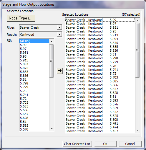
Figure 7 18. Stage and Flow Hydrograph Output Window.
As shown in Figure 7-18, the user can select individual locations, groups of cross sections, or entire reaches. Setting these locations is important, in that, after a simulation is performed, the user will only be able to view stage and flow hydrographs at the selected locations.
Flow Distribution Locations. This option allows the user to specify locations in which they would like the program to calculate flow distribution output. The flow distribution option allows the user to subdivide the left overbank, main channel, and right overbank, for the purpose of computing additional hydraulic information.
The user can specify to compute flow distribution information for all the cross sections (this is done by using the Global option) or at specific locations in the model. The number of slices for the flow distribution computations must be defined for the left overbank, main channel, and the right overbank. The user can define up to 45 total slices. Each flow element (left overbank, main channel, and right overbank) must have at least one slice. The flow distribution output will be calculated for all profiles in the plan during the computations.
Flow Roughness Factors. This option allows the user to adjust roughness coefficients with changes in flow. This feature is very useful for calibrating an unsteady flow model for flows that range from low to high. Roughness generally decreases with increases flow and depth. This is especially true on larger river systems. This feature allows the user to adjust the roughness coefficients up or down in order to get a better match of observed data. To use this option, select Flow Roughness Factors from the Options menu of the Unsteady Flow Simulation manager. When this option is selected, a window will appear as shown in Figure 7-19.
As shown in Figure 7-19, the user first selects a river, reach, and a range of cross sections to apply the factors to. Next a starting flow, flow increment, and a number of increments is entered. Finally, a roughness factor is entered into the table for each of the flows. Between the user entered flows, the model will use linear interpolation to obtain a roughness factor. If a flow is greater than the last user entered value, then that value is held constant. The user can create several sets of these factors to cover a range of locations within the model. However, one set of factors cannot overlap with another set of factors. Hence, you can only apply one set of roughness change factors to any given cross section.
Additionally, if you place these factors in both the geometry and the plan file, then you will be factoring the roughness twice. Factors placed in the geometry file get used during the Geometry Pre-Processing, and they will affect the hydraulic tables that get computed. Factors placed in the Plan file are used in real time during the unsteady flow computations, and they get applied each time step at each cross section location. 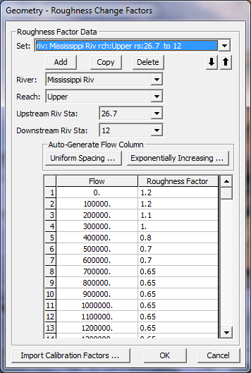
Figure 7 19. Flow versus Roughness Change Factors Editor
Seasonal Roughness Change Factors. This option allows the user to change roughness with time of year. This feature is most commonly used on larger river systems, in which temperature changes can cause changes in bed forms, which in turn causes changes in roughness. This factor can be applied in conjunction with the flow roughness change factors. When applying both, the seasonal roughness factor gets applied last. To use this option, select Seasonal Roughness Factors from the Options menu of the Unsteady Flow Simulation manager. When this option is selected a window will appear as shown in Figure 7-18.
As shown in Figure 7-20, the user first selects a river, reach, and range of river station to apply the factors to. Next the user enters the day and month in the Day column, for each time that a new roughness factor will be entered. By default the program will automatically list the first of each month in this column. However, the user can change the day to whatever they would like. The final step is to then enter the roughness change factors. During the simulation, roughness factors are linearly interpolated between the user entered values.
Figure 7 20. Seasonal Roughness Factors Editor
Automated Roughness Calibration. This option allows the user to perform an automated manning's n value calibration for an unsteady flow model. The results of this option are a set of flow versus roughness relationships, that can be applied in order to obtain a model that is calibrated from low to high flows.
To use this option, the user should first adjust the base Manning's n values (Channel and overbank values) in order to get a reasonable starting point for the automated calibration technique. The base set of Manning's n values should be within what is considered to be reasonable values for the type of river and overbank land use they are being applied to.
After a base set of Manning's n values are established, the user must break up the model into reaches for the purpose of applying and calibrating flow versus roughness factors. Once the flow versus roughness factors are set up, then the automated calibration of those reaches can be performed.
To use this option, select Automated Roughness Calibration from the Options menu of the Unsteady Flow Simulation manager. When this option is selected a window will appear as shown in Figure 7-21.
Figure 7 21. Automated Manning's n Value Editor
For a detailed discussion of the Automated Manning's n value editor and how to use this feature, please see Chapter 16 Advanced Features for Unsteady Flow Routing.
Unsteady Flow Encroachments. This option allows the user to perform an encroachment analysis using the unsteady flow simulation option. Currently, encroachments are limited to method 1 within the unsteady flow analysis module. In general the user should first perform the encroachment analysis with the steady flow computations module, as documented in Chapter 10 of this manual. Once a good steady flow encroachment analysis is completed, the final encroachments can be imported into the unsteady flow plan for further analysis and refinement. The user will need to have two unsteady flow plans, one without encroachments (representing the base flood) and one with encroachments (representing the encroached floodplain).
To add encroachments to an unsteady flow plan, the user selects Unsteady Encroachments from the Options menu of the Unsteady Flow Simulation editor. When this option is selected the following window will appear: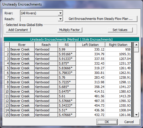
Figure 7 22. Unsteady Flow Encroachment Data Editor
As shown in Figure 7-22, the user can enter a left station and a right station for the encroachments at each cross section. Additionally, the user has the option to import the encroachments calculated from a steady flow plan. This is accomplished by pressing the button labeled Get Encroachments from Steady Flow Plan, which is shown in the upper right part of the editor. When this button is pressed the user is asked to select a previously computed steady flow plan, and a specific profile from that plan. When the user presses the OK button, the program will go and get the final computed encroachments from that particular steady flow plan and profile.
Once all of the encroachments are entered, the user presses the OK button to have the interface accept the data. However, this information is not stored to the hard disk, the user must save the currently opened plan file for that to happen. The next step is to run the unsteady flow analysis with the encroachment data. The user should have two unsteady flow plans, one without encroachments and one with encroachments. Once both plans have been successfully executed, then comparisons between the plans can be made both graphically and in a tabular format.
Ungaged Lateral Inflows. This option can be used to automatically figure out the contribution of runoff from an ungaged area, given a gaged location with observed stage and flow. The software will compute the magnitude of the ungaged area hydrograph, based on routing the upstream flow hydrograph and subtracting it from the observed downstream flow hydrograph to get the ungaged inflow contribution. This is an iterative process, in which the program figures out a first estimate of the ungaged inflow, then reroutes the upstream and ungaged inflow again, until the routed hydrograph matches the downstream observed hydrograph within a tolerance. More details of this simulation option can be found in Chapter 16 of this manual.
Computational Options and Tolerances. This option allows the user to set some computation options and to override the default settings for the calculation tolerances. These tolerances are used in the solution of the unsteady flow equations. There are separate tabs for: General; 2D Flow Options; 1D/2D Options; Advanced Time Step control; and 1D Mixed Flow Options.
When the "Calculation Options and Tolerances: option is selected, a window will appear as shown in Figure 7-23.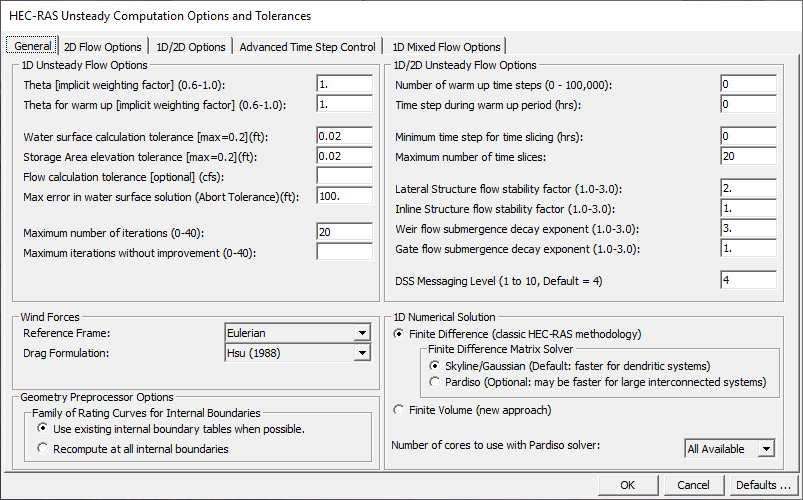
Figure 7 23 Computational Options and Tolerances with 1D Options tab shown.
The calculation options and tolerances are as follows:
General (1D Options) (see Figure 7-23):
Theta (implicit weighting factor): This factor is used in the finite difference solution of the unsteady flow equations. The factor ranges between 0.6 and 1.0. A value of 0.6 will give the most accurate solution of the equations, but is more susceptible to instabilities. A value of 1.0 provides the most stability in the solution, but may not be as accurate for some data sets. The default value is set to 1.0. Once the user has the model up and running the way they want it, they should then experiment with changing theta towards a value of 0.6. If the model remains stable, then a value of 0.6 should be used. In many cases, you may not see an appreciable difference in the results when changing theta from 1.0 to 0.6. However, every simulation is different, so you must experiment with your model to find the most appropriate value.
Theta for warm up: The unsteady flow solution scheme has an option to run what we call a "warm up period" (explained below). The user has the option to set a different value for theta during the warm up period versus the simulation period.
Water surface calculation tolerance: This tolerance is used to compare the difference between the computed and assumed water surface elevations at cross sections. If the difference is greater than the tolerance, the program continues to iterate for the current time step. When the difference is less than the tolerance, the program assumes that it has a valid numerical solution. The default value is set to 0.02 feet.
Storage area elevation tolerance: This tolerance is used to compare the difference between computed and assumed water surface elevations at storage areas. If the difference is greater than the tolerance, the program continues to iterate for the current time step. When the difference is less than the tolerance, the program can go on to the next time step. The default tolerance for storage areas is set to 0.05 feet.
Flow calculation tolerance: This tolerance is used to compare against the numerical error in the computed flow versus the assumed flow for each iteration of the unsteady flow equations. The user enters a flow in cfs (or cms in metric data sets). The software monitors the flow error at all computational nodes. If the flow error is greater than the user entered tolerance, then the program will continue to iterate. By default, this option is not used, and is therefore only used if the user enters a value for the tolerance.
Maximum error in water surface solution: This option allows the user to set a maximum water surface error that will cause the program to stop running if it is exceeded. The default value is 100 ft. If during the computations, a numerical errors grows larger than this tolerance at any node, the program will stop the simulation at that point and issue a message saying that the maximum water surface error tolerance has been exceeded.
Maximum number of iterations: This variable defines the maximum number of iterations that the program will make when attempting to solve the unsteady flow equations using the specified tolerances. The default value is set to 20, and the allowable range is from 0 to 40.
Maximum Iterations without improvement (0-40): This option allows the user to set a maximum number of iterations in which the solver can iterate without improving the answer. This option is not used by default. If turned on, it can increase the speed of the computations, but may cause larger errors or instabilities to occur if not used correctly. A good starting point for this option would be 5. What this means is, that if the program iterates five times and does not improve any of the solution errors, at all nodes in the system, then it will stop iterating and use the previous iteration that had the best answers up to that point. The premise here is that if the iteration scheme is not able to improve the solution for 5 consecutive iterations, more than likely it is not going to improve, and there is no point in wasting computational time by iterating all the way to the maximum number of iterations.
Number of warm-up time steps: Before the user entered simulation period begins, the program can run a series of time steps with constant inflows. This is called a warm-up period. This is done in order to smooth the profile before allowing the inflow hydrographs to progress. This helps to make a more stable solution at the beginning of the simulation. The default number of warm-up time steps is set to 0. This value ranges from 0 to 200.
Time step during warm-up period: During the warm-up period described in the previous paragraph, it is sometimes necessary to use a smaller time step than what will be used during the unsteady flow calculations. The initial conditions from the backwater analysis uses a flow distribution in the reaches which is often different than that computed by unsteady flow. This can cause some instabilities at the beginning of the simulation. The use of a smaller time step during the warm-up period helps to get through these instabilities. The default is to leave this field blank, which means to use the time step that has been set for the unsteady flow simulation period.
Minimum time step for time slicing: The program has an option to interpolate between time steps when it finds a very steep rise in an inflow hydrograph (see flow hydrograph boundary conditions earlier in this chapter). This option allows the user to set a minimum time step to use when the program starts reducing time steps during a steep rise or fall in flow at a flow boundary condition. This prevents the program from using to small of a time step during time slicing.
Maximum number of time slices: This option defines the maximum number of interpolated time steps that the program can use during time slicing, as described in the previous paragraph.
Lateral Structure flow stability factor: This factor is used to increase the stability of the numerical solution in and around a lateral structure. This factor varies from 1.0 to 3.0. As the value is increased, the solution is more stable but less accurate. A value of 1.0 is the most accurate, but is susceptible to oscillations in the computed lateral flow. The default value is 1.0. If you observe oscillations in the computed flow over a lateral structure, you should first check to see if you are using a small enough computation interval. If the computation interval is sufficiently small, you should then try increasing this coefficient to see if it solves the problem.
Inline Structure flow stability factor: This factor is used to increase the stability of the numerical solution in and around an Inline Structure. This factor varies from 1.0 to 3.0. As the value is increased, the solution is more stable but less accurate. A value of 1.0 is the most accurate, but is susceptible to oscillations in the computed flow. The default value is 1.0. If you observe oscillations in the computed flow over the inline structure, you should first check to see if you are using a small enough computation interval. If the computation interval is sufficiently small, you should then try increasing this coefficient to see if it solves the problem.
Weir flow submergence decay exponent: This coefficient is used to stabilize the solution of flow over a weir for highly submerged weirs. This factor varies from 1.0 to 3.0. As the headwater and tailwater stages become closer together, occasionally oscillations in the solution can occur. This exponent will prevent this from happening. The default value of one has no effect. As you increase the coefficient, dampening of the oscillations will occur. See the section called Model Accuracy, Stability, and Sensitivity later in this chapter for greater detail on this factor.
Gated Spillway flow submergence decay exponent: This coefficient is used to stabilize the solution of flow over a gated spillway for highly submerged flows. This factor varies from 1.0 to 3.0. As the headwater and tailwater stages become closer together, occasionally oscillations in the solution can occur. This exponent will prevent this from happening. The default value of 1.0 has no effect. As you increase the coefficient, dampening of the oscillations will occur. See the section called Model Accuracy, Stability, and Sensitivity later in this chapter for greater detail on this factor.
DSS Messaging Level: This option will control the amount and detail of messages that get written to the Log File when reading and writing data to HEC-DSS. A value of 1 is minimal information and a value of 10 turns on the maximum amount of information. The default for this variable is 4.
Wind Forces: This option allows you to pick a frame of reference for computing wind forces, as well as which Drag (friction) Formulation equation to use. The default Reference Frame is Eulerian, which means the speed of the wind is based on a fixed point and does not account for the direction or speed of the water. If the user selects Lagrangian, then the software will take into account the speed and direction of the water to obtain the net speed of the air over the water. The Drag Formulation allows the user to select from one of four Drag coefficient equations, or to enter a constant drag coefficient. The default is the Hsu 1988 equation. Please see the Hydraulic Reference manual for more information on these equations.
Geometric Preprocessor Options: This section of the 1D computational options allows the user to control whether or not the program will read in previously computed curves for internal boundary conditions, like bridges and culverts, etc.. Or the user can force the geometric pre-processor to recomputed all internal boundary conditions.
1D Numerical Solution: By default the 1D equation solver uses a Finite Difference scheme with a Skyline/Gaussian reduction matrix solution technique to solve the 1D Unsteady flow equations. There is an option to use the "Pardiso" matrix equation solver. We have found that even though the Pardiso solver can make use of multiple processor cores, the Skyline matrix solver is generally faster for dendritic river systems. However, for large, complex, looped systems, the Pardiso solver may produce faster computational results. The user should try the Pardiso solver is they have a larger complex system of interconnected reaches. If you turn on the Pardiso solver, there is an option to control the number of processor cores used for solving the matrix. By default, "All Available" will be used. However, the speed of the solution is sensitive to the number of cores used, and it is not always faster with using the maximum number of cores available. So user's should test the number of cores to get the maximum computational speed benefit.
A new 1D Finite Volume solution scheme has been added to HEC-RAS as an option. This numerical scheme is similar to what we do in our 2D Finite Volume solver.
The current 1D Finite Difference solution scheme has the following deficiencies:
1.Cannot handle starting or going dry in a XS
2.Low flow model stability issues with irregular XS data.
3.Extremely rapid rising hydrographs can be difficult to get stable
4.Mixed flow regime (i.e. flow transitions) approach is approximate
5.Stream junctions do not transfer momentum
The new 1D Finite Volume approach has the following positive attributes:
1.Can start with channels completely dry, or they can go dry during a simulation (wetting/drying).
2.Very stable for low flow modeling
3.Can handle extremely rapid rising hydrographs without going unstable.
4.Handles subcritical to supercritical flow, and hydraulic jumps better.
5.Junction analysis is performed as a single 2D cell when connecting 1D reaches (continuity and momentum is conserved through the junction).
However, there are some draw backs to the new 1D Finite Volume solution scheme. These deficiencies are:
1.You cannot use lidded cross sections with the new 1D Finite Volume solution scheme. Which also means that it cannot handle pressurize flow, even with the Priessman slot option turned on. If you have lidded cross sections, as soon as the water hits the high point of the lids low chord it will go unstable.
2.The 1D Finite Volume solution scheme is sensitive to the volume of water between any two cross sections. The equations are written from a "volume" perspective. If two cross sections are very close together, then there is very little volume between those two cross sections. The 1D Finite Volume scheme will require smaller time steps in order to handle the change in volume over the time step for this type of situation. The 1D Finite Difference scheme handles this better, because the equations are written in terms of change in water surface and velocity, which may be a small change for cross sections that are closer together. Therefore, for the 1D Finite Volume scheme to work well with larger time steps, users may need to remove cross sections that are very close together.
3.The 1D Finite Volume scheme is computationally slower, than the 1D Finite Difference solution scheme. This is due to the fact that the 1D Finite difference scheme combined the properties of the left and right overbank together (area, wetted perimeter, average length between cross sections, etc.) and solved the equations for a main channel and a single floodplain. The new 1D Finite Volume solution scheme keeps the left and right overbank properties completely separate. Thus the equations are written for a separate left overbank, main channel, and right overbank, and then solved. This is more computational work for every time step, but it is computationally more accurate.
2D Flow Options
When selecting the Tab labeled "2D Flow Options" on the Computational Options and Tolerances window, the editor will look like what is shown in Figure 7-24.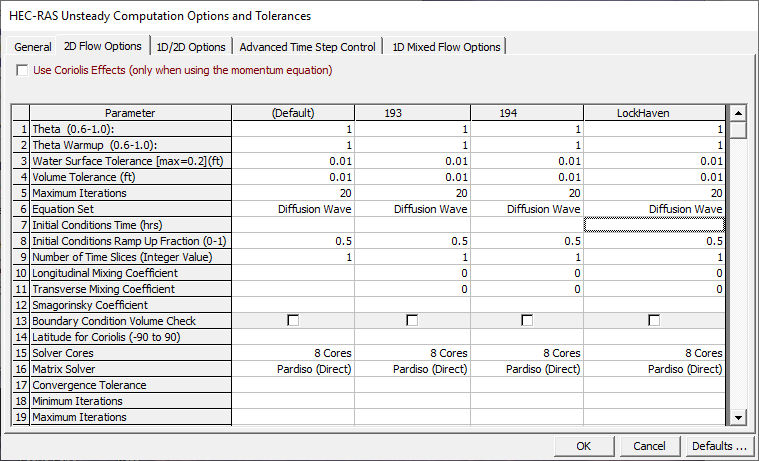
Figure 7 24 Computation Options and Tolerances with 2D Flow Area Options shown
As shown in Figure 7-24, there are several computational options and tolerances that can be set for the 2D module. These Options are discussed below.
Use Coriolis Effects: Only used in the Full Momentum Equation
This option allows the user to turn on the effects of the Earth's rotation on the solution (Coriolis Effect). When this option is turned on, the user must enter the latitude of the center of the 2D Flow Area in degrees (this is the field labeled "Latitude for Coriolis" in the table). A latitude with a value greater than zero is considered in the northern hemisphere, and a value less than zero is considered in the southern hemisphere.
Theta (0.6 – 1.0): 1.0 (default)
This is the implicit weighting factor that is used to weight spatial derivatives between the current solution time line and the previously solved solution time line. Theta of 1.0 (Default), uses only the currently solved time line for the spatial derivatives. This provides for the most stable solution, but possibly at the loss of some accuracy. Theta of 0.6, provides for the most accurate solution of the equations, but tends to be less stable. In general it has been found that in application of most real world flood runoff types of events, Theta of 1.0, will give about the same answers as Theta of 0.6. However, this should be tested for each model due to site specific geometry and flood propagation, in which it may make a difference in the results.
Theta Warm-up (0.6 – 1.0): 1.0 (default)
This is the value of Theta (see description above) that is used during the model warmup and ramp up periods. This value of Theta is only used if the user has turned on the unsteady flow warm-up option, or the Boundary Condition Ramp up Option for 2D areas.
2D water surface calculation tolerance (ft):0.01 (default)
This is the 2D water surface solution tolerance for the iteration scheme. If the solution of the equations gives a numerical answer that has less numerical error than the set tolerance, then the solver is done with that time step. If the error is greater than the set tolerance, then the program will iterate to get a better answer. The program will only iterate up to the maximum number of iterations set by the user. The default is set to 0.01 ft based on experience in using the model for a range of applications.
Maximum Number of iterations (0 – 40):20 (Default)
This is the maximum number of iterations that the solver will use while attempting to solve the equations (in order to get an answer that has a numerical error less than the user specified tolerance at all locations in the 2D computational mesh domain). The default is set to 20. However, the user can change it from 0 to 40. It is not recommended to change this unless you are sure that changing the value will either improve the chances that the model will converge (I.e. increasing the value), or speed up the computations without causing any significant errors.
Equation Set: Diffusion Wave (Default); SWE-ELM (original/faster); and SWE-EM (stricter momentum).
The HEC-RAS two-dimensional computational module has the option of running the following equation sets: 2D Diffusion Wave equations; Shallow Water Equations (SWE-ELM) with a Eulerian-Langrangian approach to solving for advection; or a new Shallow Water Equation solver (SWE-EM), that uses an Eulerian approach for advection. The new SWE equation solution method is more momentum conservative, but may require smaller time steps and produce longer run times. The default is the 2D Diffusion Wave equation set. In general, most flood applications will work fine with the 2D Diffusion Wave equations. The Diffusion Wave equation set will run faster and is inherently more stable. However, there are definitely applications where the 2D SWE should be used for greater accuracy. The good news is that it easy to try it both ways and compare the answers. It is simply a matter of selecting the equation set you want, and then running it. Create a second Plan file, use the other equation set, run it, and compare it to the first Plan for your application.
The new SWE solver (SWE-EM) is an explicit solution scheme that is based on a more conservative form of the momentum equation. This solver requires time steps to be selected to ensure the Courant number will be less than 1.0, in general (not always). This solver produces les numerical diffusion than the original SWE solver. However, in general, this new solver is only needed when user's are interested in taking a very close look at changes in water surfaces and velocities at and around hydraulic structures, piers/abutments, and tight contractions and expansions. The original SWE solver is more than adequate for most problems requiring the full momentum equation based solution scheme.
Initial Conditions Ramp up Time (hrs): Default is Blank (not used)
This option can be used to "Ramp up" the water surface from a dry condition to a wet condition within a 2D area (or from a flat water surface if an initial water surface elevation was entered). When external boundary conditions, such as flow and stage hydrographs (or 1D reaches), are connected to a 2D area, the first value of the connected flow or stage may be too high (i.e. a very large flow or a stage much higher than the cell elevation it is attached to). If the model were to start this way, such a high discontinuity could cause a model instability. This option allows the user to specify a time (in hours) to run the computations for the 2D Flow Area, while slowly transitioning the flow boundaries from zero to their initial value, and the stage boundaries from a dry elevation up to their initial wet elevation. The user specifies the total "Initial Conditions Ramp up Time" in this field (10 hours, for example). The user must also specify a fraction of this time for Ramping up the boundary conditions. A value of 0.5 means that 50% of the Initial Conditions time will be used to Ramp Up the boundary conditions to their initial values, the remaining time will be used to hold the boundary conditions constant, but allow the flow to propagate through the 2D Flow Area, thus giving it enough time to stabilize to a good initial condition throughout the entire 2D Flow Area. The Ramp up time for the boundary conditions is entered in the next row, which is labeled "Boundary Condition Ramp up Fraction".
Boundary Condition Ramp up Fraction (0 to 1.0): 0.5 (50%) Default value
This field goes along with the previous field "Initial Conditions Ramp up Time". This field is used to enter the fraction of the Initial Conditions Ramp up Time that will be used to ramp up the 2D Flow Area boundary Conditions from zero or dry, to their initial flow or stage. User's can enter a value between 0.0 and 1.0, representing the decimal fraction of the Initial Conditions Ramp up Time.
Number of Time Slices (Integer Value): 1 (Default)
This option allows the user to set a computational time step for a 2D area that is a fraction of the overall Unsteady flow computation interval. For example, if the user has set the Unsteady Flow overall computation interval to 10 minutes, then setting a value of 5 in this field (for a specific 2D area) means that the computation interval for that 2D area will be 1/5 of the overall computation interval, which for this example would be 2 minutes (e.g. 10/5 = 2). Different values can be set for each 2D Flow Area. The default is 1, which means that 2D Flow Area is using the same computational time step as the overall unsteady flow solution (computation Interval is entered by the user on the unsteady flow analysis window).
Eddy Viscosity Transverse Mixing Coefficient: Default is Blank (not used)
The modeler has the option to include the effects of turbulence in the two dimensional flow field. Turbulence is the transfer of momentum due to the chaotic motion of the fluid particles as water contracts and expands as it moves over the surface and around objects. Turbulence within HEC-RAS is modeled as a gradient diffusion process. In this approach, the diffusion is cast as an Eddy Viscosity coefficient. To turn turbulence modeling on in HEC-RAS, enter a value for the Eddy Viscosity Transverse or Longitudinal Mixing Coefficient for that specific 2D Flow Area. These coefficients require calibration in order to get at an appropriate value for a given situation. The default in HEC-RAS is zero for this coefficient, meaning it is not used. Additional diffusion using the Eddy Viscosity formulation can be obtained by entering a value greater than zero in this field. HEC-RAS also has an option to add an additional amount of turbulence using the Smagorinsky formulation.
Note: For the details on how to use the HEC-RAS Turbulence modeling, please review the section in the HEC-RAS 2D User's Manual. For information of the equations used for turbulence modeling, please review the section in Chapter 2 of the Hydraulic Reference manual.
Boundary Condition Volume Check: Default is not checked
This option is used to keep track of potential volume errors that may arise when 1D connections are made to 2D Flow Areas (i.e. Lateral structure connected from a 1D River to a 2D Flow Area). If this is turned on, the program will evaluate the volume transfer across the hydraulic connection to ensure that the volume passing over the computational time step is not more water than is truly available in the 2D Flow Area. Where this comes into play is when water is leaving a 2D flow area and going into a 1D River Reach over a lateral structure. Flow use computed by a weir equation and is based on the water surface elevations on both sides of the weir. However, there may not be enough volume left in the 2D flow area to satisfy that flow rate over the computational time step. If this option is turned on the program will make a check for this, and if the 2D Flow Area can not send that amount of water out, the software will redo the time step with a lower flow transfer rate. Turning this option on can improve the accuracy of these types of computations, but it will also slow down the computations.
Number of Cores to use in computations: All Available (Default)
The HEC-RAS two-dimensional computational module was developed from the ground up with parallel processing in mind. The HEC-RAS 2D computations will use as many CPU cores as there are available on your machine (which is the default mode for running). However, HEC-RAS provides the option to set the number of cores to use for the 2D computations. In general, it is recommended to use the default of "All Available". However, you may want to experiment with this for a specific data set to see if it will either speed up or slow down computations based on a specific number of cores. The ideal number of cores for a given problem is size and shape dependent (shape of the 2D Flow Area). As you use more cores, the problem is split into smaller pieces, but there is overhead in the communications between the pieces. So, it is not necessarily true that a given problem will always run faster with more cores. Smaller data sets (2D areas with fewer cells) may actually run faster with fewer cores. Large data sets (2D Areas with lots of cells) will almost always run faster with more cores, so use all that is available.
Shown below are the results of testing a few data sets by running them with different numbers of Cores. Each model was run several times with the number of cores set to: 1, 2, 4, 8, and 16. As you can see four of the data sets had speed improvements up to 8 cores, but actually ran slower with 16 cores. These are smaller data sets ranging from 10,000 to 80,000 cells. However, one data sets had speed improvements all the way up to 16 cores. This was the largest data set, with 250,000 cells.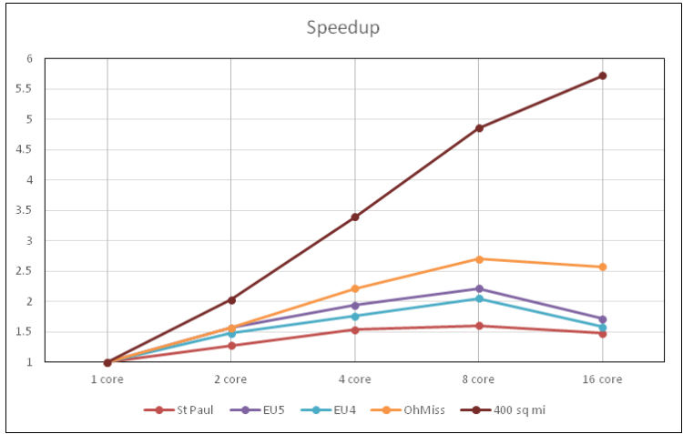
Matrix Solver. By default HEC-RAS uses a matrix solver for the 2D equations called "Pardiso". This is a direct solver. For HEC-RAS 6.0 and newer some additional "Iterative" solvers have been added. In general, the Pardiso solver produces a more stable solution. The new Iterative solvers "may" produce a faster solution (Not always), but run the risk of increasing model instability. In general user's should get ther model up and running with the Pardiso matrix solver, then they can try the iterative solvers to see if they get any performance increases with their data set.
1D/2D Options
When selecting the Tab labeled "1D/2D Options" on the Computational Options and Tolerances window, the editor will look like what is shown in Figure 7-25.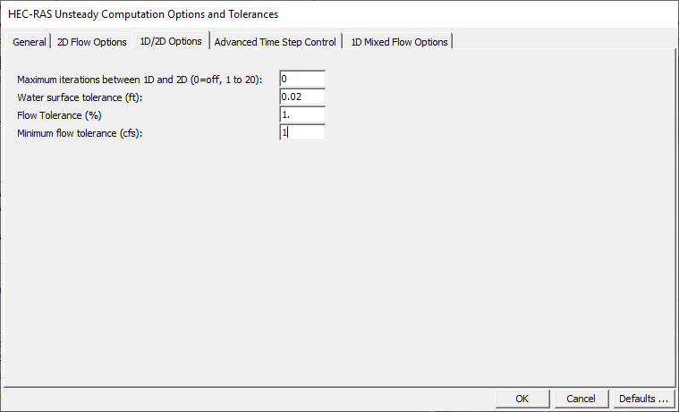
Figure 7 25 Calculation Options and Tolerances with 1D/2D Options tab shown
Maximum iterations between 1D and 2D. Default is zero (meaning this is not turned on)
There are also some options for Controlling 1D/2D Iterations, which can be used to improve the computations of flow passing from a 1D element (reach or storage area) to a 2D Flow Area. By default this option is turned off, and most 1D to 2D connections will not need iterations. However, when the1D/2D hydraulic conditions become highly submerged, or there are flow reversals, or tidally influence stages/flows, then iterating between the 1D solution and 2D solution may be necessary to get an accurate and stable answer. To turn on the 1D/2D iterations option, select the "1D/2D Options" tab. Then you can set the Maximum iterations between 1D and 2D, as well as tolerances for controlling the convergence criteria. Iteration can be set from 0 to 20, with zero meaning that it does not do any extra iterations (this is the default). In general, only use this option if you are having a stability problem at a 1D/2D hydraulic connection. Set the number of 1D/2D Iterations to as low as possible in order to get a stable answer between a 1D and 2D connection that is having stability problems. The Number of 1D/2D Iterations will cause the entire solution to be done multiple times for each time step in order to get the desired convergence. This could dramatically lengthen run times. If you turn this option on, it is suggested that you start with a low value, like 3 or so. If the stability problem still exists with that number of iterations, then increase it from there.
The convergence criteria for 1D/2D iterations consists of a Water Surface Tolerance, Flow Tolerance (%), and a Minimum Flow Tolerance. The water surface tolerance is currently only used when an upstream 1D reach is connected to a downstream 2D Flow Area. In this situation, the 1D region is computed, then the 2D region. The assumed water surface elevation at the boundary is re-evaluated. If the water surface has changed more than the Water Surface Tolerance, then the program will iterate. When the water surface elevation at the boundary has change less than the tolerance, the solution stops iterating and moves on to the next time step.
The Flow Tolerance (%) gets used for the following 1D/2D connections: Lateral Structure; SA/2D Hydraulic Connection (SA to 2D, or 2D to 2D); and 2D Flow Area to 1D Reach connection (Currently in the 5.0 Beta version, this only works when an upstream 2D flow Area is connected to a downstream 1D river reach). The default value for the Flow Tolerance (%) is 0.1 %. If 1D/2D iterations are turned on, then the flow between these types of 1D/2D connections gets recomputed after each trial to see if it has changed more than the user defined Flow Tolerance (%). If it has changed more than the flow tolerance, then the program iterates. A companion tolerance to the Flow Tolerance, is the Minimum Flow Tolerance (cfs). The purpose of this tolerance is to prevent the program from iterating when the flow passed between a 1D and 2D element is very small, and not significant to the solution. For example, you may have a connection from a 1D reach to a 2D Flow Area via a Lateral Structure, in which the flow under certain conditions is very low, so the actual change in the flow from one iteration to the next could be very small (put the percent error is very high). Such a small flow may have no significance to the solution, so iterating the entire solution to improve this small flow between the 1D and 2D elements makes no sense, and may be just wasting computational time. In general it is a good idea to set a minimum flow when turning on 1D/2D iterations. The default value is 1 cfs, however, this is most likely model specific.
Advanced Time Step Control Tab
Some new variable time step capabilities have been added to the unsteady flow engine for both 1-dimensional (1D) and 2D unsteady flow modeling. Two new options are available. One is a variable time step based on monitoring Courant numbers (or residence time within a cell), while the other method allows users to define a table of dates and time step divisors. The variable time step option can be used to improve model stability, as well as reduce computational time (not all models will be faster with the use of the variable time step). The information contained in this section is supplemental to Chapter 8 of the HEC-RAS 5.0 User's Manual.
These new Variable Time Step options are available from the Unsteady Flow Analysis window and also by going to the Computational Options and Tolerances window. There is a new button right next to the Computation Interval directly on the Unsteady Flow Analysis window, which will take users to this new feature.
When the Variable Time Step control editor ellipse button is clicked, the modified HEC-RAS Unsteady Computation Options and Tolerances window opens to the new Advanced Time Step Control tab (Figure 7-26). Alternatively, users can open the window and navigate to the new tab, from the Options | Computation Options and Tolerances menu option.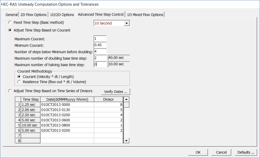
Figure 7 26. Variable Time Step Editor within the Computational Options and Tolerances.
As shown in Figure 7-26, the new Advanced Time Step Control tab now has three different methods for selecting and controlling the computational time step: (1) Fixed Time Step (default); (2) Adjust Time Step Based on Courant which is a variable time step based on the Courant number; and (3) Adjust Time Step Based on Time Series of Divisors which is a variable time step based on a user entered table of dates, times, and time step divisor's. The two new variable time step options (Courant number and Time Step Divisor) are discussed in the following sections.
Courant Number Method
The first new variable time step option is to use the Courant number method, from the new Advanced Time Step Control tab. In the example shown in Figure 7-26, the Courant number is being used for the variable time step. To use this method, select the Adjust Time Step Based on Courant option and provide the following information:
• Maximum Courant: This is the maximum Courant number allowed at any 2D cell or 1D cross section. If the maximum Courant number is exceeded, then the time step is cut in half for the very next time interval. Because HEC-RAS uses an implicit solution scheme, Courant numbers can be greater than one, and still maintain a stable and accurate solution. In general, if the flood wave is rising and falling slowly (depth and velocity are changing slowly), the model can handle extremely high Courant numbers. For these types of cases, users may be able to enter a Maximum Courant number as high as 5.0 or more. However, if the flood wave is very rapidly changing (depth and velocity are changing very quickly over time), then the Maximum Courant number will need to be set closer to 1.0. The example shown in Figure 2 6 is for a Dam break type of flood wave, in which depth and velocity are changing extremely rapidly. Because of the rapid changes in depth and velocity, the Maximum Courant number was set to 1.0.
• Minimum Courant: This is the minimum Courant number threshold for 2D cells and 1D cross sections. If the Courant number at "all" locations goes below the minimum, then the time step will be doubled. However, the time step will only be doubled if the current time step has been used for enough time steps in a row to satisfy the user entered criteria called "Number of steps below Minimum before doubling" (see below for an explanation of this field). The "Minimum Courant" value should always be less than half of the "Maximum Courant" value. If the Minimum Courant value is equal to or larger than half the Maximum Courant value, the HEC-RAS Version 5.0.4 software will just flip back and forth between halving and doubling the time steps. In the example shown in Figure 2 6, since the Maximum Courant number was set to 1.0, the minimum was set to 0.45 (less than half of the maximum), which allowed the model to stay stable, but also run faster.
• Number of steps below Minimum before doubling: This field is used to enter the integer number of time steps in which the Courant number must be below the user specified minimum before the time step can be increased. This can prevent the model from increasing the time step too quickly and/or from flipping back and forth between time steps. Typical values for this field may be in the range of 5 to 10.
• Maximum number of doubling base time step: This field is used to enter the maximum number of times the base time step can be doubled. For example, if the base computation interval is 10 seconds, and the user wants to allow it to go up to 40 seconds, then the value for this field would be 2 (i.e., the time step can be doubled twice: 10s to 20s to 40s). The value displayed in the box to the right of the user entered value is what the entered maximum time step will end up being.
NOTE: The HEC-RAS software requires that all time steps end up exactly hitting the Mapping Output Interval. This requirement is because output for HEC-RAS Mapper must be written to the output file for all cross sections, storage areas, and 2D cells at the mapping interval. Because of this fact, if users enter a "Maximum number of doubling base time step" that results in a computation interval that does not exactly land on the mapping output interval, then the unsteady flow computational program will compute its own time steps that work with the parameters entered in the Adjust Time Step Based on Courant section. Furthermore, the base time step will be changed to something close to what was entered, but when doubling it, all values will still line up with the mapping output interval. When the model runs it will list what time step it is currently using in the message window of the computational output window.
• Maximum Number of halving base time step: This field is used to enter the maximum number of time that the base computation interval can be cut in half. For example, if the base computation interval is 10 seconds, and the user wants to allow it to go down to 2.5 seconds, then the maximum number of halving value would need to be set to 2 (i.e., the time step can be cut in half twice: 10s to 5s to 2.5s). The value displayed in the box to the right of the user entered value is what the entered maximum time step will end up being.
For the Courant number method, the default approach for computing the Courant number is to take the velocity times the time step divided by the length (between 1D cross sections, or between two 2D cells). For 2D, the velocity is taken from each face and the length is the distance between the two cell centers across that face. For 1D, the velocity is taken as the average velocity from the main channel at the cross section, and the length is the distance between that cross section and the next cross section downstream.
An optional approach to using a traditional Courant number method is to use Residence Time. With this method, the HEC-RAS software is computing how much flow is leaving a 2D cell over the time step, divided by the volume in the cell. The Residence Time method is only applied to 2D cells. When this method is turned on, it is used for the 2D cells, but 1D cross sections still use the traditional Courant number approach.
User Defined Dates/Time vs Time Step Divisor
Another option available from the Advanced Time Step Control tab, is to set the variable time step control based on a user defined table of dates and times verses a time step divisor (Figure 7-26).
As shown in Figure 7-26 the user can select the option called "Adjust Time Step Based on Time Series of Divisors", from the Advanced Time Step Control tab. When this option is selected the user must enter a table of Dates and times verses time step Divisors. The first date/time in the table must be equal to the starting date/time of the simulation period. To use this method, enter a base time step equal to the maximum time step desired during the run. Then in the table, under the Divisor column, enter the integer number to divide that time step by for the current date/time in the table. Once a time step is set for a date/time, the Unsteady Flow Analysis compute will use that time step until the user sets a new one.
In the example shown in Figure 7-26, the base computational interval was set at 1 minute. Based on the table of dates/times and Divisors entered, the actual time steps that will be used are displayed in the first column labelled "Time Step".
The Time Step Divisor method for controlling the time step requires much more knowledge by the user about the events being modelled, the system being routed through, as well as knowledge of velocities, cross section spacing, and 2D cell sizes. However, if done correctly, this method can be a very powerful tool for decreasing model run times and improving accuracy.
1D Mixed Flow Options.
When this option is selected, the program will run in a mode such that it will allow the 1D Finite Difference solution scheme to handle subcritical flow, supercritical flow, hydraulic jumps, and draw downs (sub to supercritical transitions). This option should only be selected if you actually have a mixed flow regime situation. The methodology used for mixed flow regime analysis is called the Local Partial Inertia (LPI) solution technique (Fread, 1996). When this option is turned on, the program monitors the Froude number at all cross section locations for each time step. As the Froude number gets close to 1.0, the program will automatically reduce the magnitude of the inertial terms in the momentum equation. Reducing the inertial terms can increase the models stability. When the Froude number is equal to or greater than 1.0, the inertial terms are completely zeroed out and the model is essentially reduced to a diffusion wave routing procedure. For Froude numbers close to 1.0, the program will use partial inertial effects, and when the Froude number is low, the complete inertial effects are used.
Note: more information about mixed flow regime calculations can be found in Chapter 14 of the HEC-RAS User's manual.
Output Options. This option allows the user to set some additional output flags. When this option is selected a window will appear as shown in Figure 7-27. The following is a list of the available options: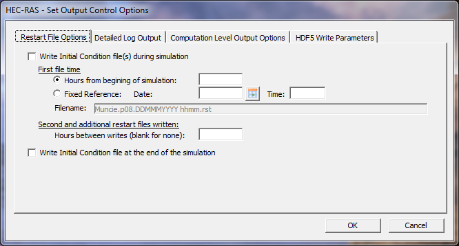
Figure 7 27. Unsteady Flow Output Control Options Window
Restart File Options: This tab allows the user to write out an Initial conditions file or files, sometimes called a "Hot Start" file. A hot start file can be used to set the initial conditions of the system for a subsequent run. This is commonly done in real time forecasting, where you want to use the results at a specific time from a previous run to be the initial conditions of the next run. The user can either enter a time in hours from the beginning of the current simulation, or they can enter a specific Date and Time. This time represents the time at which the conditions of the system will be written to the "Hot Start" file. The program writes flow and stage at all of the computational nodes, as well as the stage in all of the storage areas to the file. An additional option is available to write multiple restart files out from a single run. This is accomplished by first specifying how and when you want the first file to be written, then entering the number of hours between subsequent writes of the file. The last option of this section allows the user to ensure that the very last time step also gets written out as a separate restart file. Filenames for restart files are labeled as follows:
Projectname.p##.DDMMMYYY hhmm.rst
p##=plan number
DD=Day
MMM=Month
YYYY=Year
hh=hour
mm=minute
rst=file extension
Detailed Log Output: This tab allows the user to turn on detailed output that is written to a log file. The user can have the Input Hydrographs written to the log file; the final computed hydrographs; and they also can have the software write detailed information for each iteration of the unsteady flow equations (Write Detailed Log Output for Debugging). The detailed output at the iteration level can be written for the entire simulation period, or the user has the option to set a specific time window in which the program will only output information within this time. This option is used when there is a problem with the unsteady flow solution, in that it may be oscillating or going completely unstable. When this occurs, the user should turn this option on and re-run the program. After the run has either finished or blown up, you can view the log file output by selecting View Computation Log File from the Options menu of the Unsteady Flow Simulation window. This log file will show what is happening on a time step by time step basis. It will also show which cross section locations the program is having trouble balancing the unsteady flow equations, as well as the magnitude of the errors. There is an additional option to turn on this detailed log output only when a certain number of iterations has been met or exceeded (Automatic Detailed Log Output).
Computation Level Output: This tab allows the user to write out a limited list of variables at the computational time step level. This is a very useful tool for assisting in debugging an unsteady flow model. It is often very helpful to seem a few output variables, like water surface and flow, at the detailed computational time step in order to see when and where a model is going unstable. By default, only the water surface and the flow rate will be written out when the computational output option is turned on from the Unsteady Flow Computational window. This option allows the user to select additional variables to be written to that file. The following variables are available to be written tot the computational level output file:
WSEL=Water surface elevation (Default)
Flow=Flow rate (Default)
WS Error=Numerical error in water surface comp.
Flow Error=Numerical error in computed flow
Depth =Depth of the water from channel invert
Invert =Elevation of main channel invert
Vel Channel=Average velocity in main channel
Vel Total=Average velocity of entire cross section
Courant Chan=Courant Number for main channel only
Courant Total=Courant Number for entire cross section
Diff Eqn Parts =Separate components of the unsteady flow equations (Momentum and Continuity equations)
Friction Slope Method for Cross Sections. By default the program uses the Average Friction Slope method for determining friction forces for the momentum equation during an unsteady flow run. This option allows the user to select one of the other five available methods in HEC-RAS. To learn more about the friction slope averaging techniques in HEC-RAS, see chapter 2 of the hydraulic reference manual.
Friction Slope Method for Bridges. By default the program uses the Average Conveyance friction slope averaging technique for computing frictional forces through bridges. This has been found to give the best results at bridge locations. This option allows the user to select one of the other five available methods.
Initial Backwater Flow Optimizations. If your model has a flow split, lateral structure, or pump stations, it may be necessary to optimize the flow splits during the initial backwater computations in order to get a reasonable initial condition for the unsteady flow computations. This option allows the user to turn on flow optimizations at the various locations where flow may be leaving the system and it is a function of the water surface elevation (which would require optimization to get the right values).
Sediment Computational Options and Tolerances. As of HEC-RAS version 5.0 and newer, there is now the ability to perform Unsteady Flow Sediment Transport (deposition and erosion) computational capabilities. This Option, and the next two (called: Sediment Output Options and Sediment Dredging Options), are used to control the sediment transport computations within the Unsteady Flow computational program. Please refer to Chapter 17 for the details of performing sediment transport computations within HEC-RAS.
Check Data Before Execution. This option provides for comprehensive input data checking. When this option is turned on, data checking will be performed when the user presses the compute button. If all of the data are complete, then the program allows the unsteady flow computations to proceed. If the data are not complete, or some other problem is detected, the program will not perform the unsteady flow analysis, and a list of all the problems in the data will be displayed on the screen. If this option is turned off, data checking is not performed before the unsteady flow execution. The default is that the data checking is turned on. The user can turn this option off if they feel the software is erroneously stopping the computations from running. If this does happen the user should report this as a bug to the HEC-RAS development team.
View Computation Log File. This option allows the user to view the contents of the unsteady flow computation log file. The interface uses the Windows Notepad program to accomplish this. The log file contains detailed information of what the unsteady flow computations are doing on a time step by time step basis. This file is very useful for debugging problems with your unsteady flow model.
View Runtime Messages. This option allows the user to bring up a viewer that will show the user all of the messages that were written to the computational window for the last time the model was computed.