DLBreach can compute dam and levee breaches with a wide range of process and failure modes. Figure 4 organizes the different failure processes that DLBreach simulates into a flow chart, where the nodes represent user decisions. Figure 5 replicates this process flow chart with the actual interface options that direct these decisions in the model. 

The user decisions that direct how DLBreach computes the embankment failure include the Failure Mode (Piping or Overtopping), the Soil Type (Cohesive or Coheisonless) and, finally, the Erosion Model.
The DLBreach Erosion Model determines which process and equations (surface, composite or headcut) DLBreach will use to erode the embankment. These are overtopping algorithms, and are not used in the While DLBreach is in a piping mode. However, DLBreach will switch to these routines after the piping conduit collapses in a piping breach, so they are required for either failure mode. must be selected and the data corresponding to the selected erosion model must be entered for the breaching analysis. For all overtopping Erosion Models, users are required to enter Embankment Sediment Parameters and users have the option to Model a cover layer.

DLBreach includes three overtopping Erosion Models:

• Surface Erosion
• Headcut Erosion
• Composite (Zoned) Structure
  
  

Figure: Flow chart of the different failure models included in DLBreach. The interface options used to select these are included in a similar flow chart in the next Figure).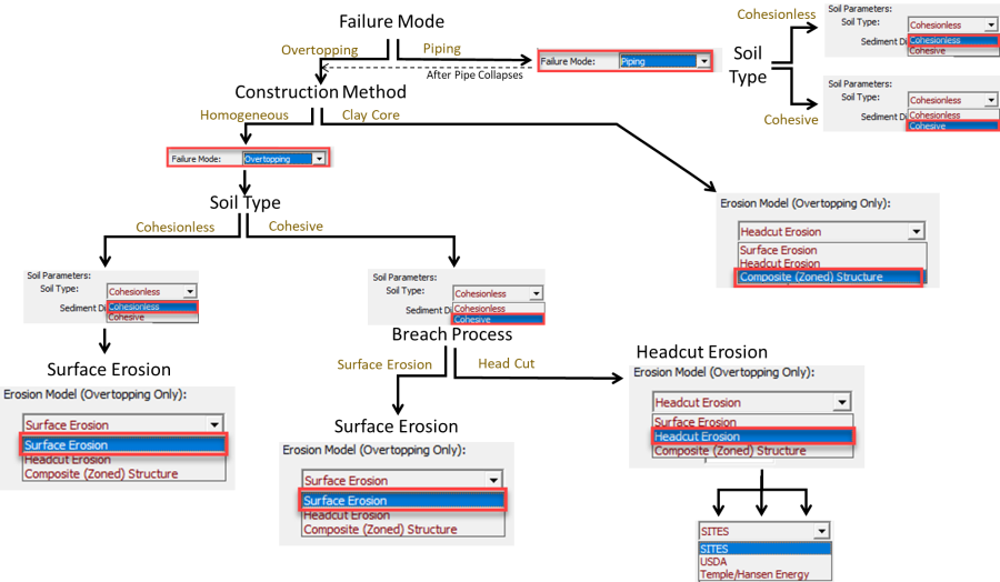
Figure: Flow Chart of HEC-RAS options to activate the different failure modes, processes, and algorithms from the previous flow chart.

Surface Erosion Model

Surface Erosion is appropriate for non-cohesive embankments or loose cohesive embankments without compaction. Therefore, HEC-RAS allows Surface Erosion with cohesive or cohesionless methods, but compacted, cohesive embankments should use the Headcut Erosion method (see next section). This method erodes sediment from the downstream slope (in a one-way breach), rotating the downstream slope around the downstream toe to account for the sediment eroded with the transport (cohesionless) or excess shear (cohesive) equation. At the same time, DLBreach lowers the flat-top weir representing the breach.Figure: Conceptual diagram of three sequential stages of a one-way Surface Erosion breach in DL Breach.

If the Surface Erosion model is selected, the model will not require additional data.

Headcut Erosion Model

Most breach experiments and field observations of actual breaches included a headcut phase. As water flows over the breach, it erodes the top of the embankment. But the flow over the breach also forms a plunge pool on the downstream end of the embankment (the Figure below), which attacks the downstream toe of the embankment, pushing the headcut upstream. DLBreach computes the headcut by idealizing the downstream face of the breach with a vertical face, and computing the rate that this vertical, downstream, embankment face translates upstream. By eroding the berm in two directions (vertically and upstream) DLBreach estimates the impact of these two interacting processes (observed in actual breaches), which adds a non-linear effect accelerating the breach. When the headcut advances to the upstream slope, the embankment crest vanishes, and the breach flow increases significantly until the upstream water surface falls.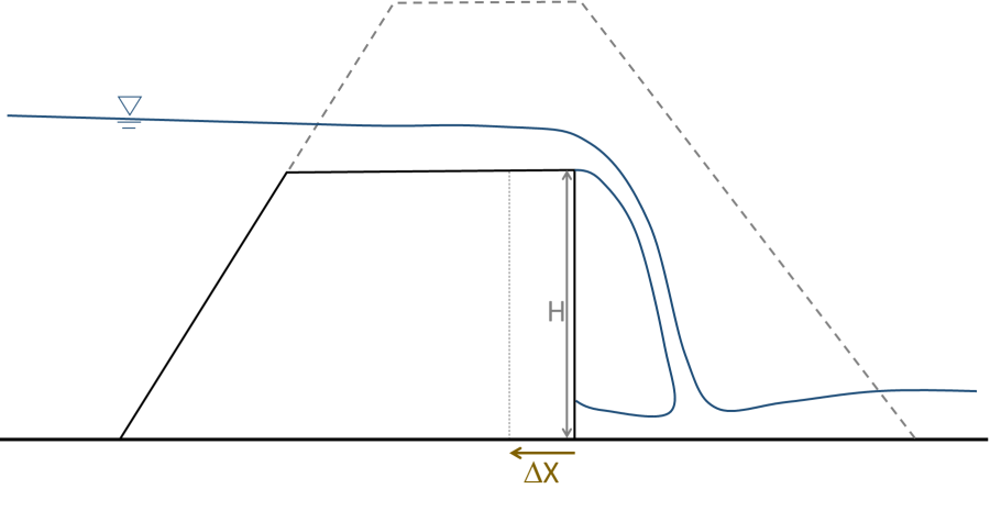Figure: Idealized headcut geometry in DLBreach. The headcut equations compute the rate of upstream erosion, which pushes the vertical downstream face of the embankment upstream by a computed X.

If modelers selects Headcut Erosion, the Headcut Method options will appear in the interface below the transport parameters.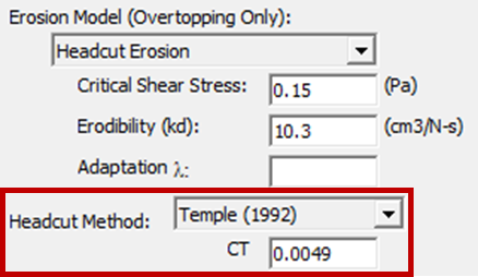

DLBreach includes three methods to compute the headcut migration. Select the method from the dropdown box next to the Headcut Method. HEC-RAS will populate one or two data fields for the parameters that these methods require. The three headcut methods available in DLBreach are:

• SITES (USDA-NECS, 1997)
• Temple (1992)
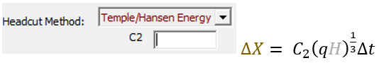
• Temple/Hansen Energy (Temple et al. 2005)

These three equations have similar forms. They all compute the rate of the headcut migration (X/t) as a function of the product of the square or cube root of the unit flow (q) through the breach and the head drop (H) over the breach, so that:
 
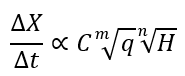
Where m and n are 2 or 3 and C is a linear, user-defined coefficient.

Temple (1992)

The 1992 Temple equation computes head cut migration the square root of the breach height and the cube root of the unit flow. Define CT to use Temple (1992) to compute headcut migration.

Temple et al. (2005)

The subsequent 2005 version of this equation is similar, except it raises both unit flow and breach height to the cube root. Therefore, the empirical coefficient has different units and behavior. Define C2 to compute headcut migration with this method.
  

SITES (USDA-NECS, 1997)

The SITES method has the same cube-root form as Temple et al (2005), but adds a threshold, computing headcut migration as the difference between the cube root of the qH product and a user defined threshold. This method requires this threshold Ao and, a linear coefficient (C1) similar to the other equations (with the same units as C2, but different behavior because of the threshold).
 

Composite (Zoned) Structure Model

Some embankments include resistant, internal cores that affect breaching processes. These cores can include internal clay, steel or concrete cores or a concrete floodwall on the crest. DLBreach includes algorithms to account for these composite structures. Breaching composite structures is a third overtopping mechanism, mutually exclusive with Surface Erosion and Headcut methods.

To simulate this process, select Composite (Zoned) Structure from the Erosion Model drop down.
This option activates the Core Data on in the right column of the editor.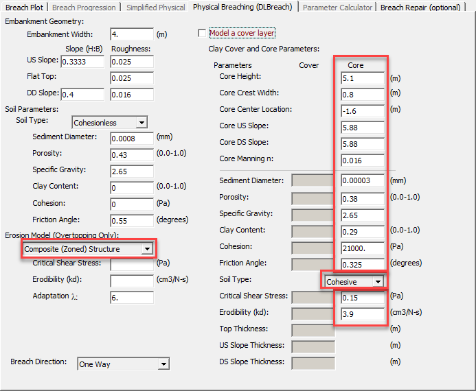Figure: Core geometry and soil parameters associated with the Composite Structure Algorithms.

In a one-way breach, the model will use the surface erosion algorithms (described above) to erode the top and downstream face of the embankment, until it encounters the core (see Figure below). DLBreach then computes erosion along the top of the core and the (steeper) downstream slope of the core using the core soil parameters highlighted in Figure 8. The example in Figure 8 uses the cohesionless surface transport equations to erode the top of the embankment and the downstream face until the clay core is exposed. When the clay core is exposed, the example in Figure 8 uses the excess shear equation to erode the cohesive material in the core. Core materials are usually less erodible than the embankment materials, but the downstream slope of the core is also, often, steeper, exposing them to higher shear stresses.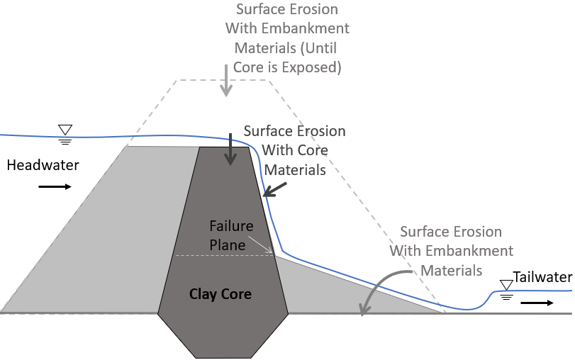
Schematic of the DLBreach approach to one-way breaching for embankments with a clay core.

At some point, however, the core can erode enough, that it becomes unstable, and fails. DLBreach evaluates the core stability each time step by balancing the forces acting on a failure plane. The failure plane is the horizontal line from the place the downstream embankment slope intersects with the core material (see figure above). 

If the driving forces on the core exceed the resisting forces, DLBreach immediately removes all of the core material above the failure plane and the upstream embankment soil above the failure plane to simulate the core failure. After a core failure, DLBreach continues to apply the surface erosion equations (cohesionless transport and/or excess shear) to erode the breach.

Core Geometry

DLBreach requires data that define the core geometry. These are in the top section of the core data column and are illustrated in the Figure below. The core geometry fields are described below: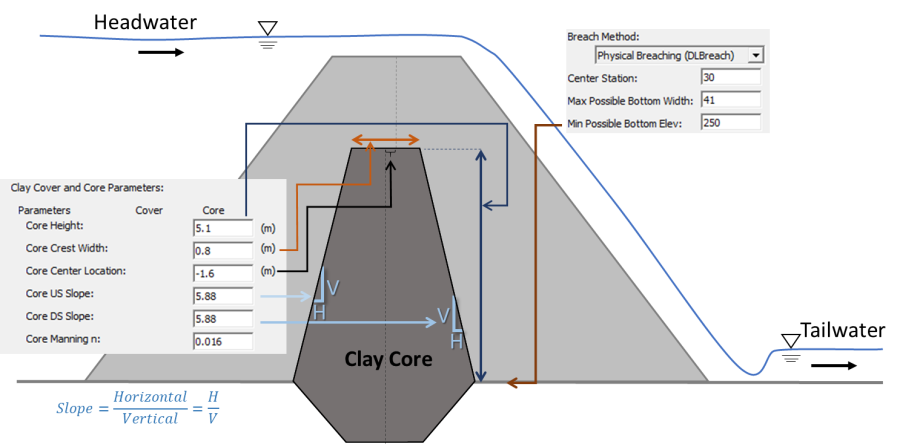Figure: The core geometry (and some related embankment geometry) data in HEC-RAS.

Core Height: The vertical distance between the Min Possible Bottom Elev in the main breach embankment editor (left panel) and the top of the core.
Core Width: The width of the flat top of the core, in the direction of flow.
Core Center Location: This is the centerline station of the core relative to the Center Station of the embankment. The stationing is based on the inline structure stationing.
Core US Slope: The upstream slope of the core (horizontal displacement divided by vertical displacement).
Core DS Slope: The downstream slope of the core (horizontal/vertical).
Core Manning n: The manning n value used to compute hydraulic parameters for surface erosion equations on the exposed core.

Core Soil Parameters

The core soil parameters are the same as the embankment soil parameters. See that section above for these parameter descriptions.

Cover

Some dams and levee include cover material that is more-or-less resistant to flow than the embankment material. DLBreach allows a cover layer with any of the erosion models. To turn on the cover layer, check the Model a cover layer option to activate the cover fields. The Cover Soil Parameters are the same as the core and embankment soil parameters. See these parameter descriptions above.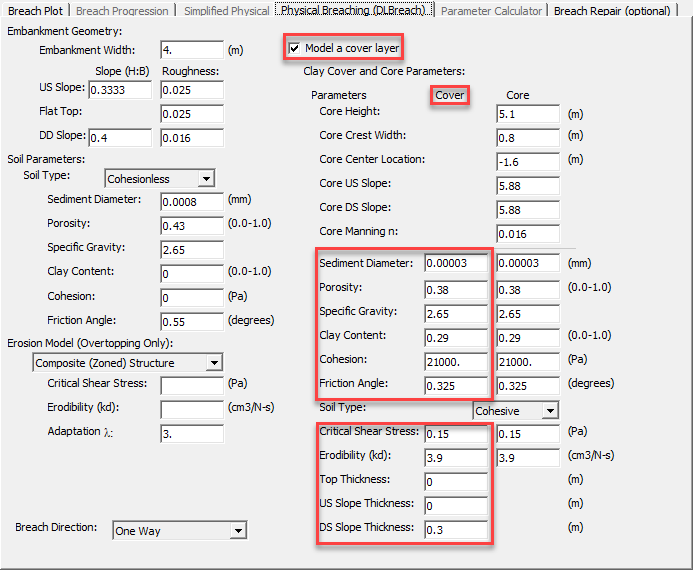Figure: Cover material parameters and local thickness.

The three data fields unique to the cover layer are all related to the cover thickens. DLBreach allows users to define separate cover thicknesses for the top of the embankment, the upstream slope and the downstream slope. These fields control those initial cover thickness as illustrated in the Figure below.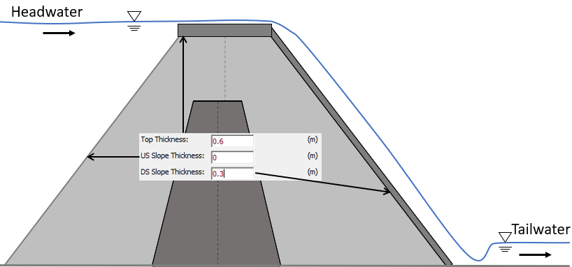Figure: Cover thicknesses in DL Breach and the HEC-RAS interface.