Boundary Conditions

All Pipe network boundary conditions (connections to the surface elements, and those defined in the Boundary Condition Editor) are applied at Nodes within the model. Pipe networks can be fully integrated with surface geometry such that all inflow and outflows for the network will be at connections to surface geometry (e.g. Drop Inlets and Culvert Openings). Conversely, pipe networks can have no surface connections at all, relying only on the defined boundary conditions in the Boundary Condition Editor. 

In the case of a pipe networks fully integrated with the surface geometry, no boundary conditions need to be explicitly defined in the Boundary Condition Editor. As long as a node is spatially contained within a surface element, it will receive inflows or outflows based on node geometry and the water surface elevations of  2D cells, Storage Area or Cross-Section to which it is connected. In the example below, rainfall is applied to a 2D Area, and a pipe network is fully integrated with the 2D Area. At the four nodes (Start and Junction Type) with defined drop inlet locations, water leaves the 2D cell and enters the pipe network. At the downstream end water leaves the pipe network and flows into a channel in the 2D Area through the Culvert Opening node.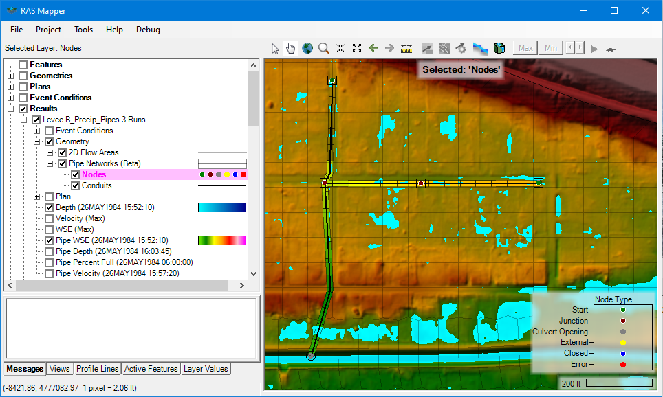

Drop Inlet Connections

Drop Inlets allow flow into and out of the pipe network based on the Drop Inlet attributes set for the node, the differences in water surface elevation between the connected surface geometry and the node. The Drop Inlet Elevation is the primary control over the drop inlet behavior, as when the water surface exceeds that elevation, flow can enter or leave the pipe network. If the Drop Inlet Elevation is higher than the Terrain Elevation then the drop inlet functions as a riser pipe. If the Drop Inlet Elevation is lower than the Terrain Elevation, flow will still be allowed into the drop inlet, but the drop inlet computations will be based on the Terrain Elevation.

Rating curves are generated from the Drop Inlet Weir Length, Drop Inlet Orifice Area, and their corresponding coefficients. The rating curves are then used to compute flows into our out of the system given the head differences between the node and the surface geometry. 

Note

In order to allow surcharge flows to leave the nodes and flow up onto the surface, drop inlets must be defined. If no drop inlets are defined and the hydraulic grade line exceeds the top of node, no flow will be allowed to leave the node as it is not connected to the surface. This means that HEC-RAS currently cannot simulate manholes with covers that prevent water from entering while still allowing surcharge overflows to exit. This is a current limitation that will be addressed in future releases. 

Culvert Opening Connections

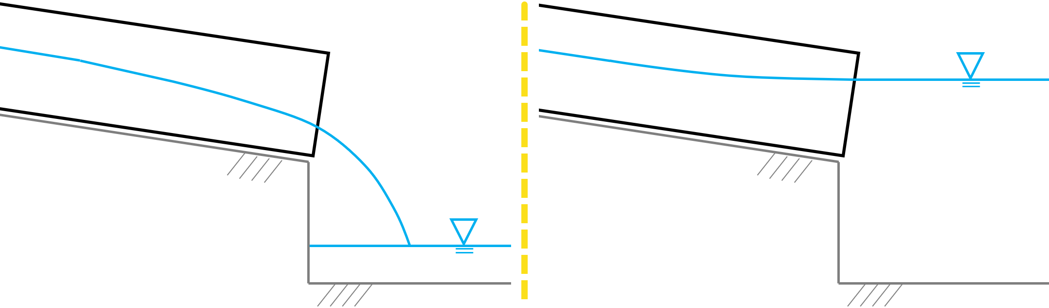
The Culvert Opening Node Type allows flow to horizontally enter or exit the pipe network from the connected 1D or 2D surface geometry element. Flow between the horizontal pipe opening and the overland area is computed using the differences between the water surface in the conduit and surface geometry element. If the conduit water surface is significantly above the water surface of the surface geometry, plunging flow is computed. When the surface water elevation rises, it will dynamically begin impacting the stages and flow in the conduit. Both of these cases are shown in the figures below.
   

User Defined Boundary Conditions

When pipe networks are not connected to surface geometry, or are partially connected to surface geometry, boundary conditions can be defined at nodes in the Boundary Condition Editor. To add boundary conditions for a pipe network, open the Boundary Condition Editor, and select Add Pipe Node... The Select Pipe Nodes Menu will appear showing all the available nodes in the model, including their System Name and Node Type.

The three types of boundary conditions that can currently be applied at nodes are Inflow Hydrograph, Normal Depth, and Stage Hydrograph. 

Stage Hydrograph - Stage Hydrographs are used to model downstream tidal or surface water boundaries, and can only be applied at External node types. Stage Hydrographs can allow flow into the pipe network, or allow flow to leave the pipe network.  If the water surface elevation in the Stage Hydrograph is higher than the node water surface elevation (or dry elevation), flow will go into the pipe network.  When the water surface elevation of the Stage Hydrograph is lower than the water surface in the pipe network, flow will leave the node cell. Note, when the full shallow water Equations are used, for the pipe network, momentum within the pipe network also impacts the computed flow leaving the pipe network.

The Stage Hydrograph boundary condition has an additional option to set the stage of the pipe network at the beginning of the simulation. If the Use Initial Stage (recommended) option is turned on, the first value in the stage timeseries will be projected into the upstream conduits and that flat water surface used as the initial condition for the simulation.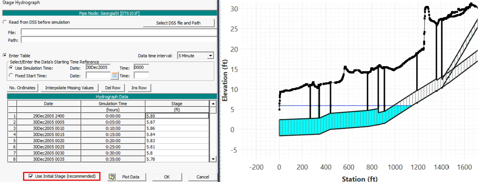

Normal Depth - Normal Depth boundary conditions are used to model free outfalls from the pipe network, and can only be applied at External node types. Normal Depth boundary conditions only allow flow out the the system using Manning's equation and a user supplied friction slope while the pipe is not pressurized. When the pipe becomes pressurized the user supplied friction slope is no longer used and instead a friction slope is computed to account for the pressure head. 

Flow Hydrograph - Flow Hydrographs are used to introduce flow into the pipe network at nodes, typically design hydrographs, or results from an external model. Flow Hydrographs can only be applied at Start, Closed, and Junction node types. Note the flow hydrographs can be connected to these nodes whether they Drop Inlet surface connections or not.

Importing EPA-SWMM Time Series Results

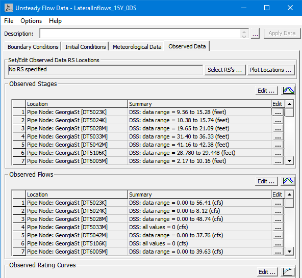
When importing an existing EPA-SWMM model for use in HEC-RAS, the results time series from the EPA SWMM model can be converted to HEC-DSS format and used as boundary conditions or observed data. 

In the unsteady flow data editor select Options → Import EPA SWMM Output As Observed.

Select the desired *.out file to be converted to HEC-DSS format. When a file is selected HEC-RAS will ask whether you would like to match the EPA-SWMM results to HEC-RAS nodes in the geometry and show the results as observed time series. If the names of the nodes in the HEC-RAS model are coincident with those from the SWMM model, new observed data locations will be created and linked to the HEC-DSS file.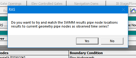

Note that the HEC-DSS file created in this process will be placed in the same directory and as the EPA-SWMM *.out file and will be given the same file name.

Simulation Options

Computational settings for the pipe networks are available in the Unsteady Computation Options and Tolerances editor. Similar to modeling with multiple 2D Areas, computation options can be set independently for each pipe network System as the run in . So a column corresponding to each pipe network system will be shown and the System Name is displayed as the column header ('Archer' in the example below).

The pipe network is computed using the same underlying solver that 2D computation engine uses and the 1D open channel finite-volume engine uses.  So the first three parameters, Theta, Water Surface Tolerance, and Volume Tolerance are the same for pipe networks as they are for 2D flow and 1D finite-volume.  An explanation of those parameters can be be found in the 2D Computation Options and Tolerances. The remainder of the parameters are discussed below. 

Adaptive Time Step - When this option is ON, the computation interval for the pipe network system is adjusted throughout the simulation by comparing the estimated residence time Courant values to the Target Courant value for each cell.  The base Computation interval set in the Unsteady Flow Plan editor will be reduced or increased until the Target Courant value is achieved for the whole pipe network system. The Default setting is ON.

Target Courant - When the Adaptive Time Step is option is ON, the computation interval for the pipe network is adjusted by so that the Target Courant value is met. The Default Setting is 0.9.

Number of Time Slices (Integer Value) - This option allows the pipe network to have a shorter time step than the base Computation Interval used for the rest of the model. For example, if the base Computation Interval for a simulation is set to 20 seconds, and the Number of Time Slices is set to 5, the pipe network computes 5 consecutive time steps (each time step being 4 seconds) after the single  (20 second) surface geometry. Note that time slicing is not available if the Adaptive Time Step is turned on. The Default setting is 1.

Maximum Iterations - The maximum number of times the pipe network solver will iterate during a given time step. The Default setting is 20.

Equation Set - The solver can use Diffusion Wave or choose between the two Shallow Water equation alternatives that include momentum terms.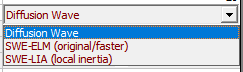

Since these are the same solvers used in the 2D computation engine, many of the same considerations apply as mentioned in the Shallow Water of Diffusion Wave Equations section of the HEC-RAS 2D User's Manual.

The Diffusion Wave solver will run faster and should be computationally more stable at longer time steps, while the Shallow Water equations will better account for momentum lost in pipe bends, expansion and contractions, and through junction boxes, but the compute is slower than Diffusion Wave. The Default setting is Diffusion Wave.

Compute Every 2D Iteration - When this option is OFF, the pipe network is computed after the connected 2D Area computation is resolved for the time step. Alternatively, when this option is ON the pipe network is computed every time the connected 2D Area iterates. This option can improve model stability and accuracy for pipe network systems that are tightly integrated with 2D areas, such as those where inflows and outflows are primarily through Culvert Openings. The increased stability occurs because as new water surface elevations in the 2D Area are updated during an iteration, the connected pipe network will be recomputed using the updated water surface elevations, and updated inflows and outflows of the pipe network. 
Default setting is OFF.

Tip

Computing Every 2D Iteration can improve overall model accuracy and stability, particularly when pipe networks are used to model culverts. However, computing a large pipe network every iteration of the connected 2D Area could significantly increase run time. 

Note

The flow out of a given 2D cell into a drop inlet is already recomputed during each 2D iteration as the depth of 2D cell changes.  The flow at the drop inlet is based on the depth in the 2D cell and the depth in the receiving pipe node. However, it is only if the pipe network is pressurized back to the surface, effectively surcharging, that the Compute Every 2D Iteration (ON) option would change the drop inlet flow during the 2D iterations.

Project Initial Water Surface from DS Surface Geometry - When ON, this option will set initial water surface elevations in the pipe network by projecting the stage from the downstream connected surface geometry upstream into the pipe network. This option prevents a surge of water entering the pipe network during the first timestep. Water surfaces will only be projected into the pipe network from downstream Culvert Opening node types. Default setting is ON

Water surface can be projected from Stage Hydrograph boundaries individually as described in User Defined Boundary Conditions.

Ramp Up Initial Water Surface from US Geometry - When ON (with a Warm Up period set) this option will establish initial conditions in pipe network by ramping up water water surface elevations from the connected surface geometry on the upstream ends of the pipe network. When the the connected upstream water surfaces are ramped up, this ramps up flows into the pipe network. This options applies to Start nodes with drop inlets, and Culvert Opening type nodes and  is intended to prevent a surge of water from entering the pipe network at the first timestep. 

Note

A Warm Up period of 30 or more timesteps must be used in combination with the Ramp Up Initial Water Surface from US Geometry option so that a sufficient period over which to ramp up water surface elevations. 

The water surface elevations applied at the pipe nodes are ramped up over the first 2/3 of the warmup period, then the applied water surface elevations are held constant for the remainder of the period. In the example below, the first 60 timesteps of the Warm Up period are used to ramp up water surface elevations applied to the pipe network, and set initial water surface elevations will be used for the remaining 30 timesteps.