To add, delete, or edit rule operations, click on the Enter/Edit Rule Operations… button at the bottom of the Rule Operations editor. This will bring up the Operation Rules editor as shown in figure 14-42.

Figure 14 42. Operation Rules Editor
Seven different types of operations can be added by clicking one of the buttons under the Insert New Operation field. A brief overview is given immediately below and this is followed by a detailed description of each rule operation type.

Operation Types

• Comment. Provides a user entered line of text (for documentation only).
• New Variable. Allows the user to create a variable and give it a custom name.
• Get Simulation Value. A variable is set equal to a given value in the simulation, such as the flow at a cross section or the time of day.
• Set Operation Parameter. Changes the operation of the hydraulic structure, for example, adjusting the gate height or setting a maximum discharge.
• Branch (If/Else). Controls which operations are executed on the basis of an If-Then test (e.g., do different gate operation checks based on seasonal considerations).
• Math. Performs math operations such as summing flows or averaging water surfaces.
• Table. This operation allows the user to enter a table and perform table lookups to get a value.

Comment

Clicking the Comment button allows the user to enter a line of text. This "operation" is not used during the computations. Rather, it is intended to make the rule set operating procedure easier to understand by allowing the user to document the rules inside of the rule set (see figure 14-43). Note: because RAS uses a comma as an internal delimiter, it will not allow a "," to be part of a comment line.

Figure 14 43. Operation Rules Editor with comment line shown

New Variable

The New Variable button brings up the editor as shown in figure 14-44. The name of the variable must be entered in the User Variable Name field. The name must be unique. That is, it can't be the same as any other variable name in the given rule set. A duplicate name will cause a run time check error, as discussed below.
By default, the variable type is real (which includes fractional numbers such as 11.35). The alternative type is integer (counting numbers such as -2, 0, 1, 5, 10, etc). If the user selects integer, the value of the variable will always be an integer. So if the current value of a user integer is 4 and a math operation (see below) adds 1.7 to it, the final value will be rounded to the nearest integer (in this case 6).
The user may enter an initial value for the variable (by default the value is zero). The variable is only initialized to this value at the start of the simulation. (To initialize a variable every timestep, use a Math operation.) It will equal this value until (or unless) it is changed by another rule. For example, if the user variable, "Test Case" has an initial value of 3 and at the start of the fourth time step it is changed (by another rule) to a value of 6. At the fifth time step, it will equal 6 (it is not "reinitialized" to 3) and will continue to equal 6 until/unless it is changed again.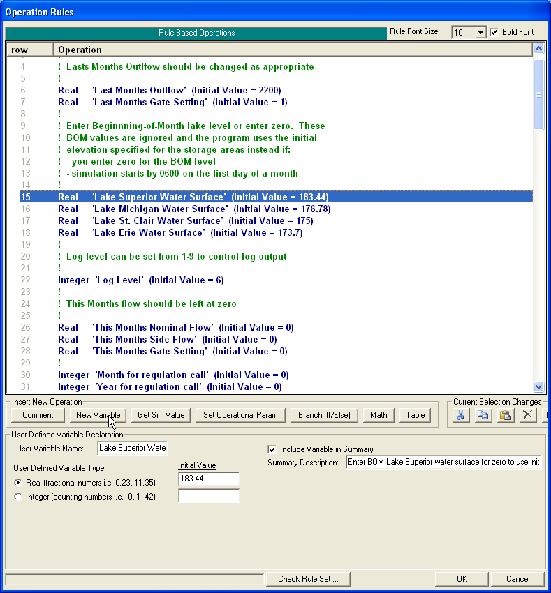

Figure 14 44. Operation Rules Editor with New Variable operation shown

If the user checks the optional "Include Variable in Summary," then the variable will be listed on the main Rule Operation editor as shown in figure 14-45. The initial value can then be entered or changed directly on the Rule Operations editor.

Figure 14 45. Rule Operations Editor with Summary of Variable Initializations

Get Simulation Value

The Get Simulation Value operation provides information about the current state of the model. In the example shown in figure 14-46, the operation is getting the day of the month at the beginning of the time step and putting it into a new variable called "Day Beg time step." For example, if the simulation time window went from 01Jan2000 to 03Jan2000 and the run was about halfway through, the "Day Beg time step" variable would be set to 2.
This is another way to create a "new variable" (a variable does not have to be created with the New Variable button). However, variables created in this manner cannot be integers (they may only be real types), they cannot be assigned an initial value (or rather, the initial value is always zero), and they cannot be included in the Variable Summary.

Figure 14 46. Operation Rules Editor with Get Simulation operation shown

If the user selected to change the Assign Result to Existing Variable, then a drop down menu would appear as shown in figure 14-47. Selecting one of the previously defined variables would put the result (day of the month in this example) into that variable instead of creating a new one.

Figure 14 47. Get Simulation Value assigning to an existing variable

Note: on renaming New/Existing variables. A new variable (whether it is from a user variable, get simulation, math, or table operation) can be renamed by typing in a new name. However, any references to that variable will not be automatically renamed! A reference to a non-existent variable will result in a run time check error. The user will have to manually change all references to that variable (whether on the Assign Result to an Existing Variable or using an Existing Variable in an Expression, see below). This is also covered in the discussion of Check Rule Set, below.

There are currently eight categories of simulation variables (more may be added later). These are Time, Solution, Cross Section, Inline Structure, Lateral Structure, Storage Areas, Storage Area Connectors, and Pump Stations. Clicking on the "+" will expand the list for that category. A complete list and definition of each variable is given at the end of this section of the manual.
For all the variables under Time, the user can select to use the time at the beginning of the time step (default), the end of the time step, or the previous time step. For example, assume the time step was 30 minutes long and the program had just finished the time step that ended at 12:15 (the program had just gone from 11:45 to 12:15 and was getting ready to go from 12:15 to 12:45). The minute of the hour at the beginning of time step would be 15. The hour of the day (fractional) for the beginning of the time step, end of time step, and previous time step would be 12.25, 12.75, and 11.75, respectively. The hour of the day at both the beginning and end of the time step would be 12. The previous hour of the day would be 11.

To get a water surface or flow at a normal cross section, expand the Cross Section list and highlight either the Flow or WS Elevation field as shown in figure 14-45. This will also display the standard node selector to allow the user to select the river, reach and river station for the desired cross section (also shown in figure 14-48).

Figure 14 48. Selecting water surface at a cross section

At the far right is another drop down menu that allows additional choices for when and how the simulation value (water surface in this example) is computed, see figure 14-49. The default is the Value at the current time step. In the time example above, this would be the water surface at 12:15 for river station 73.75. Alternately, the user could select the Value at previous time step, which would be the water surface at 11:45 in the above example.

Figure 14 49. Changing how simulation values are computed

The remaining choices provide various options for the value further back in time. Selecting Value at specified lag, will display a window where the lag time in hours is specified. So continuing to build on the same example, a lag time of 1.5 hours would get the water surface at the given cross section at 10:45 (12:15 minus 1.5 hours equals 10:45). For the next four options, the user must specify a starting and ending lookback time. Selecting Sum over previous time window, the user could enter 1.5 for the starting time and 0 for the ending time (for the specified time window to end at the current time step, the ending time should be 0). So if the user selected flow, this would sum the flow for the previous 1.5 hours. In other words, it would return the volume of water passing the given node for the previous 1.5 hours (since the value takes into account the length of each time step, this is more technically an integral instead of a sum). Or the user could select water surface, select Average over the previous time window, enter 2 hours for starting time and 1 hour for ending time, see figure 14-50. This would return the average water surface at the cross section between 10:15 and 11:15. The next two options will return either the maximum or minimum value over the given user specified time window (e.g. the highest water surface).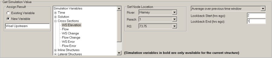

Figure 14 50. One hour average water surface starting two hours ago

Under the inline structure simulation variables as shown in figure 14-51, some of the choices are shown in bold font. The variables shown in bold are user settable operational parameters (Figure 14-52) for the current hydraulic structure (which happens to be an inline structure). These variables are also provided under the Get Simulation Value. This provides a way to check what an operational parameter has been set to (if it has been set at all). So, for instance, if a maximum flow had been set for the structure, then the Structure – Flow Maximum variable would return the value that this had been set to. The variables listed in bold are only available for the current inline structure—this is the hydraulic structure that this particular rule set is attached to.)

Figure 14 51. Getting an Operational Parameter

Set Operational Parameter (for hydraulic structures)

Clicking the Set Operational Param button brings up the editor that allows a change to be made to the hydraulic structure operations (i.e. adjusting a gate opening).  Changes can only be made for the hydraulic structure or pumping station that the rule set is attached to.  This is the hydraulic structure (inline, lateral, or storage area connection) that was selected on the Unsteady Flow Data editor.

Figure 14‑52. Setting an Operational Parameter

Figure 14-52 shows a change being made to the gate opening height (the gate will be moved to the new gate setting based on the Opening/Closing rate and maximum and minimum values, if any).  If a gate variable is used, the appropriate gate group must be selected from the drop menu at the bottom.  The new value is set equal to the value of the expression.  (The expression might be a constant, such as the number “5”, a user variable as shown in Figure 14-52, or a simple math operation.  See Math operations, below, for a detailed description of using expressions).  The Opening Rate or Closing Rate changes the rate at which the gate can open or close.  This overrides any value that the user may have entered on the Rule Operations editor.

Gate - Flow (Fixed) sets the gate flow to the given value.  However, setting or changing the Flow (Fixed) value does not affect the gate opening height (the given amount of flow will be released through this gate group from the reservoir regardless of the gate opening height).  The Fixed flow value will be used each time step until the Fixed flow is changed or removed.  To remove the Gate - Flow (Fixed) parameter, set the Flow (Fixed) expression to “Not Set” as shown in figure 14-53 (see Math below for editing expressions).

Figure 14‑53. Turning off the Gate Fixed Flow

Gate - Flow Maximum and Minimum puts limits on the gate flow.  For example, if the user sets the flow maximum to 1000 cfs, the program would first compute the flow through the given gate based on the gate opening and water surface(s), if the flow is below 1000, it would use that value.  If the computed flow was larger, the program would restrict the flow to the user entered amount (1000 cfs).  Note, however, that the Gate Maximum and Minimum flow will not override a Gate Fixed flow value.  Gate Maximum and Minimum flow can be removed by using the “Not Set” value.

Gate - Flow (Desired) will cause the program to adjust the gate opening in order to give the given, desired, flow (based on the water surfaces and the gate characteristics) through the gate group.  Once the gate opening is determined, the program will use this opening height to compute the actual flow.  Since determining the gate opening is an inexact, iterative process, the actual computed flow may not perfectly match the desired flow.  Note also that the program will not open/close the gates faster than the current Opening/Closing Rate, if any, allows.  The program will adjust the gate opening each time step as long as the Gate Flow Desired has a value.  This feature can be turned back off by using the “Not Set” value.  Having the Desired value on will not prevent the final gate flow from being overwritten by a Maximum, Minimum, or Fixed flow.  If the user wishes to force a given gate flow, but also wishes to know the [approximate] gate settings that would result in that flow, then this can be done by setting both the Fixed flow and the Desired flow to the same value (e.g. 3000 cfs).

The rule set shown in figure 14-54 illustrates how these gate features can be used and combined.  The resulting output is shown in figure 14-55.

Figure 14‑54. Desired and Fixed Flow Gate Operations

The initial gate opening is 6.0 feet.  The If/Then test on row #2 is false until the time reaches 1:15 (this is 1.25 in fractional hours).  At that point, row #4 is executed and the Desired Flow is set to 600 cfs.  The gates open (at the user set opening rate) until the flow is approximately 600 cfs.  After 1:30, the Desired Flow is turned off (“not set”).  The gates then remain at that, current, gate height (6.1295 feet).  At 1:45 row #8 is executed and the flow is fixed at 700 cfs (but the gate opening height is not changed).  At 2:30, the Desired Flow is turned back on by setting it to 700 cfs (same as the fixed flow).  This causes the gates to adjust.  However, the actual release remains exactly 700 cfs because the Fixed Flow is still set to 700.

Figure 14‑55. Output from Desired and Fixed Flow Gate Operations

In addition to the gate control operations for individual gate groups, the user can set limits on all of the gates groups combined:

Structure - Total Gate Flow sets the flow for all of the gate groups.  Instead of summing the flow from each gate group (and regardless of whether the gate group flow is “natural” or “fixed”), this flow is used instead.

Structure - Total Gate Flow Maximum sets a maximum flow for all of the gate groups.  It will not override Structure - Total Gate Flow.

Structure - Total Gate Flow Minimum sets a minimum flow for all of the gate groups.  It will not override Structure - Total Gate Flow.

The next category of structure operation parameters are for weirs:

Weir – Flow fixes the amount of flow over the weir.

Weir - Flow Maximum sets the maximum flow over the weir.  It will not override Weir – Flow.

Weir - Flow Minimum sets the minimum flow over the weir.  It will not override Weir – Flow.

Weir - Weir Coefficient sets the weir coefficient for the weir.  (Tip:  this allows a straight forward way to adjust the weir coefficient based on the depth and/or velocity of flow over the weir).

Weir - Minimum Elev for Weir Flow changes the minimum weir elevation that is required before the program will compute flow for the weir.

Weir - C Simple (Positive) sets the linear routing coefficient for positive flow (linear routing weirs only).

Weir - C Simple (Negative) sets the linear routing coefficient for negative flow (linear routing weirs only).

The final category of structure operation parameters are for the overall structure:

Structure - Total Flow (Fixed) forces the given flow for the inline structure.  This flow is used regardless of the flow from the gates and/or weir.

Structure - Flow Maximum sets a maximum flow for the inline structure.  It will not override the structure Fixed flow.

Structure - Flow Minimum sets a minimum flow for the inline structure.  It will not override the structure Fixed flow.

Structure - Flow Additional will add in the additional given flow to the inline structure.  It will not override the structure Maximum, Minimum, or Fixed flow.

Structure - Total Flow (Desired) computes gate settings to provide the total given flow for the inline structure.  It works in a similar manner to Gate - Flow (Desired).  However, it will open or close any/all of the gate groups to get the correct flow.  (To increase flow, gate groups are opened in a left to right manner.  To decrease flow, gate groups are closed from right to left.)  Weir flow (and Flow Additional) is included in the desired flow (if the desired flow is 2000 cfs and the weir flow is 500 cfs, the gates will be adjusted to get 1500 cfs of flow).  Structure - Total Flow (Desired) will not override Structure - Total Flow (Fixed).  However, it will still adjust the gate group settings.

Structure - Stage (Fixed) will force the given water surface immediately upstream of the inline structure.  This option is very similar to the stage part of the Internal Boundary (IB) Stage and Flow Hydrograph option from the Unsteady Flow Data editor (see chapter 8).  When the Unsteady Solver determines all of the flows and water surfaces at all the cross sections during the solution of a given time step, it will compute the amount of flow at the inline structure that is required in order to produce the given water surface.  It is easy to generate instability and/or hydraulically unrealistic flows when using this option.  For instance, a large increase in the fixed stage over a single time step could potentially cause very small or even negative flows through the inline structure and/or cause the model to go unstable.  A large drop in the fixed stage may generate a flow that is physically greater than the structure is capable of passing.  To avoid these problems when changing the given water surface, it is recommended that the fixed stage is gradually adjusted over a period of time.  In the sample data sets that are included in the HEC-RAS installation, there is an example that illustrates this.

It should be noted that the Fixed Stage option is not compatible with the other set operational parameters.  The flow through the inline structure is completely controlled by the requirement to generate the correct, given water surface.  Therefore, any maximum, minimum, and/or fixed flow rules, that would otherwise be in effect, are ignored.  Additionally, when the Fixed Stage rule is being used, HEC-RAS will automatically adjust the gates (and will also ignore any set operations for the gate openings).  The gates are adjusted in order to approximate the gate opening that would be needed to accommodate the computed flow.  Effectively, a Total Flow (Desired) rule is put into effect where the desired flow is set equal to the flow that is being forced through the structure by the Fixes Stage option.  This will generally allow the Fixed Stage option to be turned off (using the “not set” feature) and normal gate flow to be resumed without causing instability.

Set Operational Parameter (for pumping stations)

Clicking the Set Operational Param button for pumping station brings up the editor shown below (figure 14-56).

Figure 14 56. Setting an Operational Parameter for Pumping Stations

The operation of rules to control a pumping station is generally similar to the operation of rules to control a hydraulic structure, but, there is at least one notable difference. If a Rules Boundary Condition is selected for a hydraulic structure, then all of the control of that structure (e.g., gate openings) is handled by the Rules entered from the Operation Rules Editor.
However, this does not have to be the case for a pumping station. When a Rule Set is entered for a pumping station, the Rule Operation could be used in order to modify the control of the pumping station without entirely superseding the information that was entered as part of the geometry. For example, a pumping station may have a set of rules that determine a maximum amount that can be pumped, but the rules do not specify when the pumps should be turned on and off. This results in a hybrid control situation. Whether the pumps are pumping or not is determined from the data entered as part of the geometry. The amount of pump flow is also determined from the pump efficiency curve from geometry information, but this amount is not allowed to exceed the maximum set by the rules.
Alternately, the user can override the geometry control by the use of rule operations. But even after the rules have superseded the geometry, the rules can still "hand control" back to the geometry control. This brings up an important concept about the control of a pumping station.
When using rules, there are two fundamentally different modes of operation for turning individual pumps on and off.
Initially, the pumps are turned on and off based on the WSEL On and WSEL Off elevations that have been entered in the Geometry Pump Station Data editor. This is referred to as the WSEL On and Off mode of operation. (That is, this mode is active.) The pump rules can be used to modify the water surface elevations (the water surface elevations entered from the geometry) that the pumps turn on and off. This does not, in itself, change the WSEL On and Off mode. If the mode was active, it stays active.
However, a pump can also be turned on or off by directly using a rule. Anytime a rule is used to turn a pump on or off, then the WSEL On and Off mode is automatically deactivated for that pump. When the WSEL On and Off mode is deactivated, the On/Off water surfaces elevations (that were entered as part of the geometry) will no longer control that specific pump. (The pump can continue to be turned on and off using rule operations, of course.) If it is desired to return control to the On/Off water surfaces on the geometry editor, then the WSEL On and Off mode must be made active. This is done by using the Reactivate WSEL On and Off mode rule (see below).

Station – Pump Flow sets the pumping station flow to the given value.

Station – Pump Flow Maximum sets a maximum flow for the pumping station.

Station – Pump Flow Minimum sets a minimum flow for the pumping station.

Station – Turn All Pumps On starts turning all the pumps on (this will make the WSEL On and Off mode inactivate for all pumps).

Station – Turn All Pumps Off starts turning all the pumps off (this will make the WSEL On and Off mode inactivate for all pumps).

Group – Pumps Flow sets the group pump flow to the given value.

Group – Pumps Flow Maximum sets the maximum group pump flow to the given value.

Group – Startup Time sets the time to ramp on the pumps in this group to the given value.

Group – Shutdown Time sets the time to ramp off the pumps in this group to the given value.

Group – Flow Factor sets a multiplier for the pump flow in this group to the given value.

Group – Head Maximum sets a maximum head this group will pump against.

Group – Head Minimum sets a minimum head this group will pump against.

Group – Additional Head sets an additional head this group will pump against.

Group – Turn All Pumps On starts turning all the pumps in this group on (this will make the WSEL On and Off mode inactivate for pumps in this group).

Group – Turn All Pumps Off starts turning all the pumps in this group off (this will make the WSEL On and Off mode inactivate for pumps in this group).

Pump – Flow sets the pump's flow to the given value.

Pump – Flow Maximum sets the pump's maximum flow to the given value.

Pump – Flow Minimum sets the pump's minimum flow to the given value.

Turn Pump On starts turning the pump on (this will make the WSEL On and Off mode inactivate for this pump).

Turn Pump Off starts turning the pump off (this will make the WSEL On and Off mode inactivate for this pump).

Reactivate WSEL On and WSEL Off mode this will make the WSEL On and Off mode activate for this pump. The pump will turn on and off based on the water surface elevations entered on the Geometry Pump Station Data editor.

WSEL On sets the water surface elevation to turn this pump on (when the WSEL On and Off mode is active for this pump).

WSEL Off sets the water surface elevation to turn this pump off (when the WSEL On and Off mode is active for this pump).

Branch (If/Else):

The branching Branch(If/Else) operation allows for decision making based on the value of two (or four) expressions. Figure 14-57 shows a simple example. If the gate flow is less than 500 cfs, then the program will go from row #4 to the next operation at row #5. Otherwise, it will skip down to the first row after the End If (row #7). Note that the editor automatically indents the operations between the If and the End If.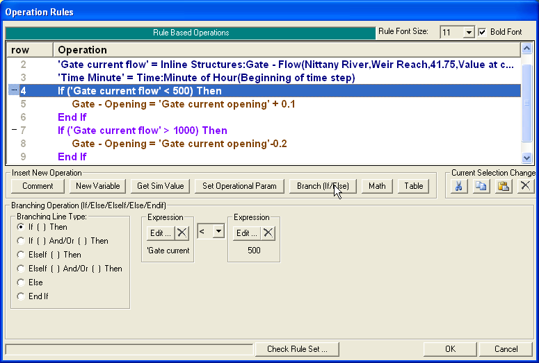

Figure 14 57. Branching Operations

Clicking the Branch(If/Else) button brings up a blank (i.e. not set) If/Then as shown in figure 14-58. The user must define a value for both expressions. Going back to figure 14-57, the first expression is the flow through the gate and the second expressions is the constant 500. The user must also choose a comparison test from the drop down menu between the two expressions. In figure 14-57 (row #4), the comparison is less than. So the If/Then test is true when the first expression is a smaller number than the second (i.e., the flow is under 500 cfs). The comparisons that the user can choose from are: less than, less than or equal to, greater than, greater than or equal to, equal to, or greater than or less than (i.e. not equal to).

Figure 14 58. Creating a (blank) If/Then Operation

The user must add the End if that is associated with each If/Then. This is done by clicking on the Branch(If/Else) which brings up another blank If/Then as shown in figure 14-59. For the Branching Line Type, select End If as shown in figure 14-60.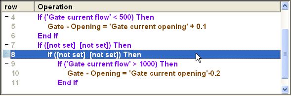

Figure 14 59. Adding another blank If/Then Operation (first step in adding an End if)

Figure 14 60. Changing the Branching Line Type to an End if

Important! There must be one, and only one, End If for each If/Then.
The rule set as shown in figure 14-59 is not valid because it has three If/Then operations but only two End Ifs. Notice how the last operation, row #10, is indented. If the last row is indented, then the rule set is missing at least one (if not more than) End if.

Although not required, it is highly recommended that the user create the End If operation immediately after adding the If/Then operation.
When the If/Then is added (figure 14-59), all the remaining operations are indented, which can look confusing. Figures 14-59 and 14-60 show the steps in adding the End if. To add the End If, the Branch(If/Then) is clicked again, which adds another If/Then that causes the remaining operations to be indented even further (figure 14-58). However, once the rule operation is changed from an If/Then to an End If (figure 14-59) the remaining operations return to their appropriate location. With the desired If/Then and End If in place, the If/Then operation can be defined and additional rule operations can be inserted between the If/Then and the End If as desired. The program will allow the operations to be added in any order. So the user could, of course, create the If/Then and then add the additional operations, before finally creating the End If. However, up until the End If is added, the indentation on the display is liable to cause confusion.

Warning! When an If/Then rule operation is deleted, the user must also delete the appropriate End If.
Just as it is possible to have more If/Then operations than End If operations, it is also possible to have too many End If operations. There is an erroneous End If in row #7 of figure 14-61 (if there is an End If that does not have an If/Then, it will be displayed in red). If a rule set has a large number of operations with complex, nested If/Then operations, it may be worthwhile to note which End If corresponds to which If/Then before beginning to delete either rule operation.

Figure 14 61. Erroneous "End If" is displayed in red

Instead of simple If/Then, a two part if test can be done by selecting the If And/Or Then option under the Branching Line Type. This requires the user to define four expressions and select a logical operator, figure 14-62. In the first part, the first two expressions are compared (using a greater than for the example in figure 14-62). In the second part, the third and fourth expressions are compared (using a less than or equal to, in the example). The final step is testing the two parts with the logical operator. For figure 14-62, And has been selected from the drop down menu between the two sets of expressions. If both the first part and the second part are true, then the overall If test is true. If either, or both, the first or second part are false, then the overall If test will be false. The two parts can also be tested with an Or logical operator by changing the selection on the drop down menu. If this is done, the test will be true if either the first or the second part is true. Only if both parts are false will the If test then be false.

Figure 14 62. Two part If/Then test

If/Then operations can be nested. Figure 14-63 shows an example where the check for the gate adjustment is made at the top of the hour and half past the hour. If the first If/Then is false (not an appropriate time), then control will jump to after the corresponding End If (as shown by the level of indentation) at row 12. Continuing the example, If the first If/Then is true (time to make flow check) then the second If/Then will be evaluated (row #5). Control will go to row #6 or row #8 depending on whether the second If/Then is true or false.

Figure 14 63. Nested If/Then test

After an If/Then and corresponding End If have been added, an Else can be added as shown in figure 14-64. When the original If is false, control will go to the first line after the Else (row #12 in the example). When the original If is true, the operations between the If and the Else will be performed. Once control reaches the Else, it will jump to the End If (after row #10 control will jump to row #14).

Figure 14 64. Else Operation

Instead of a simple Else, another option is an ElseIf. In this case, there is a second conditional. The operations after the ElseIf will only be performed if the initial If is false and the second If (that is, the ElseIf) is true. Additional ElseIfs can be added as shown in figure 14-65. An Else can also be combined with the ElseIf(s). However, there can only be one Else and it must come after the ElseIf(s). Therefore, after a simple Else operation, there may not be any more ElseIf or Else operations. (The limitations on ElseIfs/Else only apply to branching types at the same level of indentation, that is, in the context of the given If/Then End If. There may still be other "nested" conditionals with their own ElseIfs and Else operations).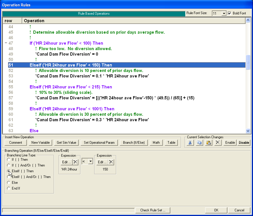

Figure 14 65. Elseif Operations

The display of the rule operations between an If/Then and the corresponding End If may be "collapsed." Note the "" at the beginning of each If/Then rule. Clicking the "" will change it to a "" and the display of the rules between the If/Then to End If will collapse as shown in figure 14-66. These rules are still in effect (collapsing rules does not change their operation). This option merely changes the display, and it is intended to make large rule sets easier to understand and manage. Clicking the "" will expand the rules back to their original form. Note: all of the operations under the Current Selection Changes (cut, copy, paste, etc), see below, function normally even on collapsed regions. In the above example where the collapsed region is highlighted, clicking the Delete button would delete rules 47 through 66.

Figure 14 66. Collapsed If-Then

Math

Clicking the Math operation button creates a [blank] math operation as shown in figure 14-67.  The result of the math operation can be assigned to either a new variable or an existing variable (in the same way that a get simulation variable can be assigned, as above).

The math operation itself is composed of up to four different “expressions.”  Each expression that is defined will return a real number.  Expressions should be defined from left to right.  So if a math operation is composed of two expressions, the left two expressions should be defined and the right two expressions should be left as “[not set]” (i.e. they should be left blank).  If more than one expression is defined, then the user must choose an algebraic connector from the drop down menu between them.  The choices are:  addition, subtraction, multiplication, and division.

The value of each individual expression is determined and then the remaining algebraic operations are performed from left to right.  So if the math operation has the three expressions as shown in figure 14-68, the first two expressions are added together and that sum is then divided by the third expression.

Figure 14‑67. Blank Math Operation

Figure 14‑68. Three Expression  Math Operation

Expression.  To define an expression, click on the Edit button to bring up the Edit Rule Expression editor as shown in figure 14-69.  If no values have been entered (or if the Clear Expression button has been clicked), then the current expression will be shown as “[not set].”

Figure 14‑69.  Blank Rule Expression

Up to five fields in the expression editor can be defined.  Any that are not defined are ignored.  The simplest expression is to enter a single number in the Constant field as shown in figure 14-70.  In this example, this expression will always have a value of 5.

Figure 14‑70.  Rule Expression set to a constant

Another simple example is shown in figure 14-71.  Here a preexisting variable has been selected from the drop down menu.  This expression will return the current value of this variable.  An optional coefficient can be added in front of the selected variable and a value may also still be added under the constant field.

Figure 14‑71. Rule Expression set to an existing variable

The Variable can also be raised to an exponent by entering a value in either or both of the fields inside of the parenthetical.  If only the Exponent Coefficient or the Exponent Variable is defined, then the variable is raised to the given value of the Exponent Coefficient or Exponent Variable, see figure 14-72.  If both are defined, then the Exponent Variable is multiplied by the Exponent Coefficient and the given Variable is raised to the resulting product.

Figure 14‑72. Variable raised to an exponent multiplied by a coefficient

Note:  each expression is always determined before operations between expressions are performed.

Table

The final operation type is a table lookup.  Clicking the Table operation button creates a table operation as shown in figure 14-73.  The result of the table lookup can be assigned to a new variable or an existing variable.  The table can be either one or two dimensional.

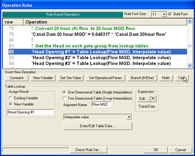
Figure 14‑73. Table lookup operations

Figure 14-73 shows a one dimensional table operation.  The table data can be entered (and/or viewed) by clicking on the Enter/Edit Table Data… button.  This brings up the Rule Table editor as shown in figure 14-74.

Figure 14‑74. Rule Table Editor

When the table operation is performed, the program will determine the value of the Expression, which starts out ‘Canal Dam’ in the example in figures 14-73 and 14-74.  The location of the Expression value is determined in the left hand column of the table (figure 14-74) and the corresponding lookup value is determined from the right hand column.  In the above figure, if the value of the expression happens to equal 13.08, the result of the table lookup would be to assign the value 1.2 to the variable “Head Opening #1.”

The Argument Name (“Flow MGD” in the above example) is used as the heading for the left column.  This is only used as a label.  (Alternately, the program could have used the numeric formula in the given expression as the heading label, but this could be rather long and awkward.)  This label is only used as a heading in the Rule Table editor (it is not a user selectable variable).

The right hand column is labeled with the assignment result.  In this example, the result of the table lookup is being assigned to a new variable called “Head Opening #1.”

By default, the lookup will interpolate between values.  So in the above example, if the expression equaled 14.78, the lookup would return 1.3.  This can be changed by the drop down menu that is just above the Enter/Edit Table Data.  There are three other choices.  “Nearest index value” will move up or down to the nearest value (14.7 would return 1.2 and 14.8 would return 1.4, in the above table).  “Index <=value” and “Index >=” will go down or up to the next value in the table.  These other options can be useful for forcing exact gate settings.  For instance, if it was desired that the gates only be opened to the nearest tenth of a foot, values in tenths (e.g., 3.0’, 3.1’, 3.2’, etc) could be entered in a table and “Nearest index value” selected.  The result of the table lookup could then be used to set the gate.

Tip:  Another possibility for forcing exact gate settings is to use an integer user variable.  Assume that the gate can be opened in hundredths of a foot (e.g., 3.00’, 3.01’, 3.02’, etc.).  These could be [tediously] entered into a table.  Alternately, the approximate gate opening could be determined, say for example, 3.028 feet.  This value could be multiplied by 100 to get 302.8.  This value, 302.8 could be assigned to an integer user variable which would result in 303.  Finally, this could be divided back by a 100 (assigning the result back to a real variable) to get 3.03 that could then be used to set a gate opening.

NOTE:  By default the software will extrapolate at both ends of the user entered tables.  Meaning, if a value is requested above the last value of the Table, the software will take the last two points in the table, project a straight line, and then extrapolate to get a value.  The same thing is done at the lower end of the table.  If a value is requested that is below the lowest point in the table, the first two vales are used to create a straight line, and a value is extrapolated below the table.  Therefore if you want to control the lower end of the table, you will need to put in an extra row that will encompass all possible values requested.

Instead of a one dimensional table, the other option is a two dimensional table as shown in figure 14-75.  The editor now has two expressions and two argument Names (the top argument name corresponds with the left expression and the bottom argument name corresponds with the right expression).  Clicking Enter/Edit Table Data brings up an expanded Rule Table as also shown in figure 14-75.  As before, the left most column corresponds to the value in the first expression.  The top row now corresponds to the second expression.  The value in the table is determined by two way interpolation (or nearest value depending on the interpolation option).  So in the table shown, if the first expression (“Inline Flow”) is equal to 5000 and if the second expression (“Hour”) is equal to 9, then the value from the table lookup would be 400.

Figure 14‑75. Two dimensional Table

Current Selection Changes.  On the right hand side of the Operation Rule editor (figure 14-76), are six buttons for manipulating the current, highlighted rule (or selection of rules).  The Cut, Copy, Paste, and Delete buttons operate in a normal, Windows manner.  One or more rules may be selected using the keyboard (e.g. Shift + down arrow) or the mouse pointer (e.g. Ctrl + click) as shown in figure xxx.  A copy of the rule(s) can be put on the Clipboard with the Copy button and can then be pasted (using the Paste button) to another location, as shown in figure 14-80.

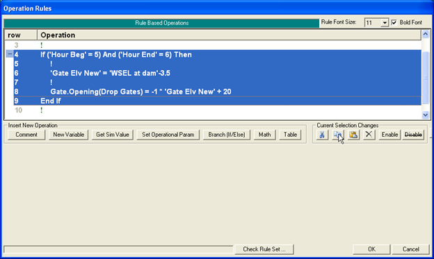
Figure 14‑76. Copying Highlighted Rules

The copy function makes an exact duplicate of the selected rules.  This can generate potential “errors” that the user will have to correct.  For instance, in the above example of using the copy function, rule 6 is a Get operation that assigns the result to the “New Variable” named Gate Elv New.  The copy of this rule, rule 13 in figure 14-77, is also assigning the result to the same “New Variable” named Gate Elv New.  After copying this rule, the user must change one of the “Gate Elv New” names to something else.  Or, if it is intended that the copy use the same variable, the user should change the assign result for the copied rule to “Existing Variable” and then select Gate Elv New from the drop down menu.

Since the copy function uses the standard Windows Clipboard, rules can be pasted into a completely different rule set, or the user can even open up a different plan (or different RAS project) and paste the results.  The user will have to correct any erroneous variable names or references (different cross section river stations, different gate group names, etc.).

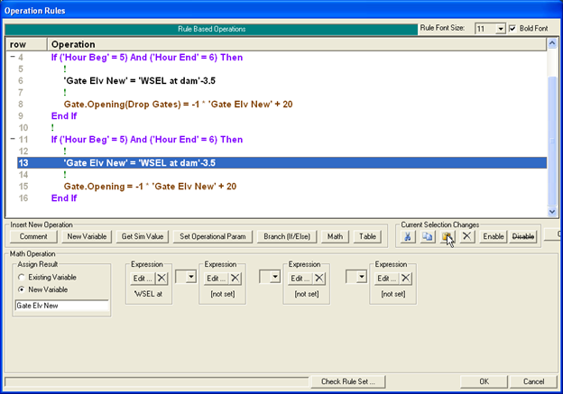
Figure 14‑77. Pasting Rules

The Cut button will move the highlighted rule(s) to the clipboard.  After the rules have been removed by cutting, the Paste button can then be used as a “move” operation.  The Delete button permanently removes the highlighted rules.  There is no “undo” operation, so care should be exercised when using the Delete button.  However, if a mistake is made, the Cancel button will cancel all the changes that have been made since the Operation Rules editor was opened.  Tip:  frequently saving the changes made in the Operation Rules editor allows the Cancel button to be used as an “undo” operation without canceling too much work.

Note:  If a collapsed If/Then-End If block is highlighted, then it will still be subject to copy, paste, and delete/cut, just as it would be in its fully expanded state.

Tip:  The standard Windows shortcut keys:  Ctrl + “x”, “c” or “v” may be used instead of clicking on the Cut, Copy, or Paste buttons.

Checking the Disable button is a quick way to temporarily remove the highlighted operations (it will cause the highlighted operations to be displayed as green comment lines with a strikethrough), see figures 14-78 and 14-79.  These operations will no longer be performed by the program (be careful disabling Branching Line Types).  Clicking the Enable button will restore the operations.

Figure 14‑78. Disabling Highlighted Rules

Figure 14‑79. Disabled Rules

The Copy Rules Text to Clipboard will copy the display text of the entire rule set to the clipboard (figure 14-80).  This can then be pasted, for instance, as simple text into Notepad or a Word document report (figure 14-81).  This copy if for “display” only and may not be pasted back into a rule set.

Figure 14‑80. Copying Rule Text to the Clipboard

Figure 14‑81. Text Pasted into Notepad

Clicking the right mouse button (on a given row) will display a popup editor as shown in figure 14-82.  In addition to the functions described above, the Insert New Operation functions are also available in this manner.

Figure 14‑82.  Right mouse click on a line

Clicking the Check Rule Set… button will cause RAS to check the rule set for common user errors.  All of the rule sets in the model will also be checked when an unsteady flow run is launched.  The Check Rule Set… button is just a convenient way to find and fix rule errors for the given rule set while the Operation Rules editor is opened.

If no errors are found, RAS will display a message stating that no inconsistencies were found.  Otherwise, RAS will display a list of the mistakes and the line numbers they occur.  An example is shown in figure 14-83.  Common problems are:  a variable name that has been defined more than once, a reference to a non-existent variable (the variable was renamed or deleted), “unbalanced” If/Then End If operations, or a reference to a non-existent node (e.g. a river station that has been removed from the project).

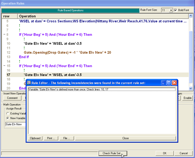
Figure 14‑83. Checking the Rule Set

Font.  In the upper right hand corner of the Operation Rule editor, there is a drop down menu where the user can change the rule operation font size.  The font can also be toggled between normal and bold by checking the Bold Font box.

Detailed Log Output.  If the detailed log output is turned on, then results from each rule set will be sent to the log file during runtime, see figure 14-84.  On the left side is the row number of the operation followed by the result of the operation.  For instance, the operation at row #19 results in the variable ‘Tampa Dam Flow’ being set equal to 324.9499.  Row #32 is an If/Then test that came back false.  For this time step, for this operation, the first and second expressions are both equal to 4.  This results in the less than or greater than (i.e. ‘not equal to’) test being false.  Since the test is false (and there is not a corresponding ElseIf or Else), control jumps to after the End If, which happens to be row #121.  Row #121 is a two part If/Then test that is also false.  It is expected that additional, (tabular and graphical) output from rule set operations will be added to future versions of HEC-RAS.  For the current version of RAS, the log output may be the best way to track down user programming mistakes.  Rule operations that are valid (as far as RAS is concerned), but do not produce the result desired by the user.  For instance, a Get operation that references the wrong cross section node.

Figure 14‑84. Detailed log output

Simulation and Operational Variables. 

The following is a list of the currently available simulation output variables and operational variables that can be set.

Time variables

Julian Day:  Days since December 31, 1899 (e.g. 01Jan2000 = 36525).

Year:  Year (e.g. 2006).

Month: Month of the year (e.g. August = 8).

Day of Year:  e.g. Jan 1 = 1. Feb. 1 = 32.  Dec 31 is 365 (non-leap year).

Day of Water Year:  e.g. Oct 1 = 1.  Sept 30 = 365 (non-leap year).

Day of Month:  e.g. 22Jan2000 = 22.

Day of Week:  Integer day starting on Sunday. e.g. Sunday = 1, Monday = 2, Saturday = 7.

Hour of Day:  Integer hours since midnight (e.g.  01Jan2000 1245 = 12).

Minute of Hour:  Integer minutes after hour (e.g.  01Jan2000 1245 = 45).

Second of Minute:  Integer seconds after minute (e.g.  01Jan2000 1245:15 = 15).

Hour of Day (fractional):  (fractional) Hours since midnight (e.g.  01Jan2000 1245 = 12.75).

Hour of Simulation:  (fractional) Hours since simulation started.

Solution variables

Time Step:  Length of current time step in hours.

Iteration Number:  Number of iterations, for given time step (“current time step” will not have relevance until rules are allowed for every iteration, see above, but “previous time step” will return the number of iterations from the last time step).

WS Error Max:  Maximum error, for given time step, in computed water surface at any cross section (“current time step” will not have relevance until iterations are allowed, see above, but “previous time step” will return the maximum error from the last time step).

Flow Error Max:  Maximum error, for given time step, in computed flow at any cross section (previous time step only).

WS SA Error Max:  Maximum error, for given time step, in computed water surface at any storage area (previous time step only).

Cross Sections variables

WS Elevation:  Water surface.

Flow:  Flow.

WS Change:  Change in water surface, for given time step (previous time step only).

Flow Change:  Change in flow, for given time step (previous time step only).

WS Error:  Error in water surface, for given time step (previous time step only).

Flow Error:  Error in flow, for given time step (previous time step only).

Bed Change:  The change in elevation of the thalweg (only applicable for Unsteady Sediment simulations).

Sediment Concentration:  The concentration of sediment leaving the cross section (only applicable for Unsteady Sediment simulations).

Inline Structures, Lateral Structures, and Storage Area Connections variables:

Structure - Total Flow:  Total flow for the inline structure.

Structure - Total Flow (Fixed):  Force the given flow for the inline structure.

Structure - Total Flow (Desired):  Compute gate settings to provide the total given flow for the inline structure.

Structure - Flow Additional:  Add in the additional given flow to the inline structure.

Structure - Flow Maximum:  Set a maximum flow for the inline structure.

Structure - Flow Minimum:  Set a minimum flow for the inline structure.

Structure - Total Gate Flow:  Flow for all of the gate groups.

Structure - Total Gate Flow Maximum:  Set a maximum flow for all of the gate groups.

Structure - Total Gate Flow Minimum:  Set a minimum flow for all of the gate groups.

Structure - Stage (Fixed):  Sets the given stage.  Computes the flow through the inline structure that is required to produce the given stage.

Weir - Flow:  Flow over the weir.

Weir - Flow Maximum:  Set a maximum flow over the weir.

Weir - Flow Minimum:  Set a minimum flow over the weir.

Weir - Weir Coefficient:  Weir coefficient for the weir.

Weir - Minimum Elev for Weir Flow:  Minimum weir elevation for flow for the weir (water surfaces below this elevation will not produce weir flow).

Weir - C Simple (Positive):  Linear routing coefficient for positive flow (linear routing weirs only).

Weir - C Simple (Negative):  Linear routing coefficient for negative flow (linear routing weirs only).

Weir - Submergence:  Fractional submergence for the given weir (e.g. 0.97).

Gate - Flow:  Flow through the gate group.

Gate - Flow (Fixed):  Force the given flow for the gate group.

Gate - Flow (Desired):  Compute gate setting to provide the given flow for the gate group.

Gate - Flow Maximum:  Set a maximum flow through the gate group.

Gate - Flow Minimum:  Set a minimum flow through the gate group.

Gate - Opening:  The [current] gate opening height for the gate group.

Gate – Opening (target position):  Gate target opening height set by user/rule.  If the user has specified a new gate opening (by using the rules), but this gate opening has not yet been reached because of constraints in how fast the gate can open or close, then this variable will be the new, target opening.  If no target position has been specified, then this variable will be the current gate opening height.

Gate - Submergence:  (fractional) Gate submergence for the gate group (e.g. 0.88).

Gate - Opening Rate:  Gate opening rate for the gate group.

Gate - Closing Rate:  Gate closing rate for the gate group.

Lake Superior (Plan 1977A):  This get simulation value will determine the nominal monthly outflow for Lake Superior as specified by the Plan 1977A regulations.  This computation is based on the value of user defined variables that must be in a specific order.  The first twelve rule operations (excluding comment lines) must be defined in the order show in figure 14-41.

Storage Areas variables

WS Elevation:  Water surface elevation for the given storage area.

Net Inflow:  Net inflow for the given storage area (e.g. Total Inflow - Total Outflow).

Total Inflow:  Total inflow for the given storage area (gross inflow, ignores outflow).

Total Outflow:  Total outflow for the given storage area (gross outflow, ignores inflow).

Area:  Current surface area of storage area.

Volume:  Current volume of storage area.

Pump Stations variables:

Station – Pump Flow:  Total pump flow for the pump station.

Station – Pump Flow (transition complete):  What the total pump flow would be (at current heads) when all pumps have finished ramping on or ramping off.  If there are no pumps that are currently ramping on or off, then this variable will equal Station – Pump Flow.

Station – Pump Flow Maximum:  Set a maximum flow for the pumping station.

Station – Pump Flow Minimum:  Set a minimum flow for the pumping station.

Station – Turn All Pumps On:  Starts turning all the pumps on.

Station – Turn All Pumps Off:  Starts turning all the pumps off.

Station – WSEL Inlet:  Water surface at pump inlet.

Station – WSEL Outlet:  Water surface at pump outlet.

Station – WSEL Reference:  Water surface at the reference node (as defined on the Geometry Pump Station Data editor).

Group – Pump Flow:  Total pump flow for the pump group.

Group – Pump Flow (transition complete):  What the total pump flow would be (at current heads) when all pumps in this group have finished ramping on or ramping off.  If there are no pumps that are currently ramping on or off, then this variable will equal Group – Pump Flow.

Group – Pump Flow Maximum:  Set a maximum flow for the pump group.

Group – Startup Time:  Sets the time to ramp on the pumps in this group.

Group – Shutdown Time:  Sets the time to ramp off the pumps in this group.

Group – Flow Factor:  Sets a multiplier for the pump flow in this group.

Group – Head Maximum:  Sets a maximum head this group will pump against.

Group – Head Minimum:  Sets a minimum head this group will pump against.

Group – Additional Head:  Sets an additional head this group will pump against.

Group – Turn All Pumps On:  Starts turning all the pumps in this group on.

Group – Turn All Pumps Off:  Starts turning all the pumps in this group off.

Group – Number of Pumps On:  The number of pumps in this group that are on.  Any pumps in the process of ramping off will not be included.

Pumps On (fraction):  A decimal fraction that represent whether this pump is on or off or transitioning.  This value is 0.0 when the pump is fully off, it is 1.0 when fully on, and it is a fraction between  0.0 and 1.0 when it is ramping on or off.

Pump – Flow:  Pump flow.

Pump – Flow (transition complete):  What the pump flow would be (at current heads) when this pump has finished ramping on or ramping off.  If the pump is not currently ramping on or off, then this variable will equal Pump – Flow.

Pump – Flow Maximum:  Set a maximum flow for the pump.

Pump – Flow Minimum:  Set a minimum flow for the pump.

Turn Pump On:  Starts turning the pump on.

Turn Pump Off:  Starts turning the pump off.

Reactivate WSEL On and WSEL Off mode:  This will make the WSEL On and Off mode activate for this pump.

WSEL On:  Sets the water surface elevation to turn this pump on (when the WSEL On and Off mode is active for this pump).

WSEL Off:  Sets the water surface elevation to turn this pump off (when the WSEL On and Off mode is active for this pump).