Download PDF
Download page 2D Flow Areas.
2D Flow Areas
![]()
Two Dimensional Flow Areas (2D Flow Areas) are regions of a model in which the flow through that region will be computed with the HEC-RAS two dimensional flow computation algorithms. 2D Flow Areas are defined by laying out a polygon that represents the outer boundary of the 2D Flow Area. Then the user must define the computational mesh.
2D Flow Area can be located at the beginning of a reach (as an upstream boundary to a reach), at the end of a reach (as a downstream boundary to a reach), or they can be located laterally to a reach. 2D Flow Areas can be connected to a river reach by using a lateral structure connection. 2D Flow Areas can be connected to another 2D Flow area or a Storage Area by using a SA/2D Area Connection (this is described later in this chapter).
The HEC-RAS 2D modeling capability uses a Finite-Volume solution scheme. This algorithm was developed to allow for the use of a structured or unstructured computational mesh. This means that the computational mesh can be a mixture of 3-sided, 4-sided, 5-sided, etc… computational cells (up to 8 sided cells). However, the user will most likely select a nominal grid resolution to use (e.g. 200 X 200 ft cells), and the automated tools within HEC-RAS will build the computational mesh.
The HEC-RAS 2D meshing capability is unique to HEC-RAS, however, the mesh can be created using other software and used within HEC-RAS 6.x. This includes using meshes developed with HEC-RAS 2025. A tutorial on using a RAS25 mesh is available here: Importing a HEC-RAS 2025 Mesh.
For a more detailed description of how to use the HEC-RAS two-dimensional modeling capabilities, please see the separate 2D Modeling User's Manual.
Note:
A 2D Flow Area, and computational mesh, is developed in the HEC-RAS Geometry editor by doing the following:
Draw a Polygon Boundary for the 2D Flow Area
The user must add a 2D flow area polygon to represent the boundary of the 2D area using the 2D flow area drawing tool in the Geometric Data editor (just as the user would create a Storage Area). The best way to do this in HEC-RAS is to first bring in terrain data and aerial imagery into HEC-RAS Mapper. Once you have terrain data and various Map Layers in RAS Mapper, they can be displayed as background images in the HEC-RAS Geometry editor. Additionally, the user may want to bring in a shapefile that represents the protected area, if they are working with a leveed system. The background images will assist the user in figuring out where to draw the 2D flow area boundaries in order to capture the tops of levees, floodwalls, and any high ground that will act as a barrier to flow.
Use the background mapping button on the HEC-RAS Geometry editor to turn on the terrain and other Map Layers, in order to visualize where the boundary of the 2D Flow Area should be drawn.
For levees and roadways this is obviously the centerline of the levee and the roadway. However, when using a lateral structure to connect a main river to the floodplain (when there is no actual levee), try to find the high ground that separates the main river from the floodplain. Use this high ground as a guide for drawing the 2D boundary, as well as defining the Lateral Structure Station Elevation data.
To create the 2D Flow Area, use the 2D Flow Area tool (the button on the Geometric Editor Tools Bar labeled 2D Flow Area, highlighted in red on Figure 12). Begin by left-clicking to drop a point along the 2D Flow Area polygon boundary. Then continue to use the left mouse button to drop points in the 2D Flow Area boundary. As you run out of screen real-estate, right-click to re-center the screen. Double-click the left mouse button to finish creating the polygon. Once you have finished drawing the 2D area polygon by double clicking, the interface will ask you for a Name to identify the 2D Flow Area. Shown in Figure 5-41 is an example 2D Flow Area polygon for an area that is protected by a levee. The name given to the 2D Flow Area in this example is: "2D Interior Area".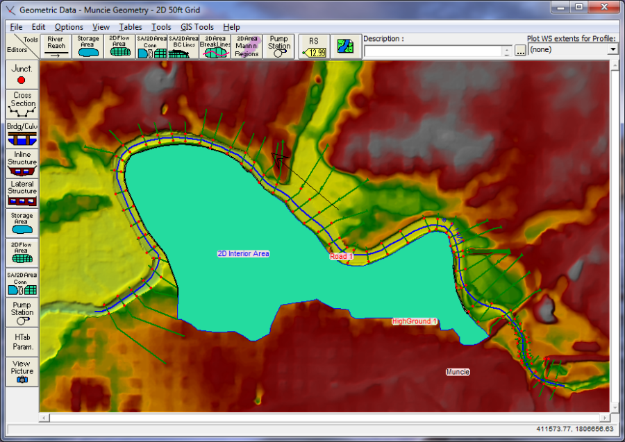
Figure 5 41. Example 2D Flow Area polygon.
Adding Break Lines inside of the 2D Flow Area
Before the computational mesh is created the user may want to add break lines to enforce the mesh generation tools to align the computational cell faces along the break lines. Break lines can also be added after the main computational mesh is formed, and the mesh can be regenerate just around that break line. In general, break lines should be added to any location that is a barrier to flow, or controls flow/direction.
Break lines can be imported from Shapefiles (GIS Tools/Breaklines Import from Shapefile); drawn by hand; or detailed coordinates for an existing breakline can be pasted into the break line coordinates table (GIS Toools/Breaklines Coordinates Table). To add break lines by hand into a 2D flow are, select the 2D Area Break Line tool (highlighted in Red in Figure 3-2), then left click on the geometry window to start a break line and to add additional points. Double click to end a break line. While drawing a breakline, you can right click to re-center the screen in order to have more area for drawing the breakline. Once a break line is drawn the software will ask you to enter a name for the break line. Add break lines along levees, roads, and any high ground that you want to align the mesh faces along. Break lines can also be placed along the main channel banks in order to keep flow in the channel until it gets high enough to overtop any high ground berm along the main channel.
Creating the 2D Flow Area Computational Mesh
Select the 2D Flow Area editor button on the left panel of the Geometric Data editor (Under the Editors set of buttons on the left) to bring up the 2D Flow Area editor window: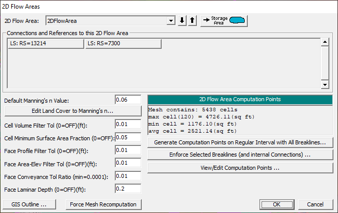
Figure 5 42. 2D Flow Area Mesh Generation Editor
The 2D Flow Area editor allows the user to select a nominal grid size for the initial generation of the 2D flow area computational mesh. To use this editor, first select the button labeled Generate Computational points on regular Interval …. This will open a popup window that will allow the user to enter a nominal cell size. The editor requires the user to enter a Computational Point Spacing in terms of DX and DY (see Figure 3-5). This defines the spacing between the computational grid-cell centers. For example, if the user enters DX = 50, and DY = 50, they will get a computational mesh that has grids that are 50 x 50 everywhere, except around break lines and the outer boundary. Cells will get created around the 2D flow area boundary that are close to the area of the nominal grid-cell size you selected, but they will be irregular in shape.
Since the user can enter break lines, the mesh generation tools will automatically try to "snap" the cell faces to the breaklines. The cells formed around break lines may not always have cell faces that are aligned perfectly with the break lines. An additional option available is Enforce Selected Breaklines. The Enforce Selected Breaklines option will create cells that are aligned with the breaklines, which helps ensures that flow cannot go across that cells face until the water surface is higher than the terrain along that break line. When using the Enforce Selected Breaklines option, the software will create cells spaced along the breakline at the nominal cell size entered buy the user. However, the user can enter a different cell spacing to be used for each breakline. This is accomplished by selecting GIS Tools/Breaklines Cell Spacing Table, and then entering a user defined cell spacing for each breakline.
The popup editor has an option to enter where the user would like the cell centers to start, in terms of an upper left X and an upper left Y coordinate. These Starting Point Offset fields are not required. By default it will use the upper left corner of the polygon boundary that represents the 2D flow area. Use of the Shift Generated Points option allows the user to shift the origin of the grid cell centers, and therefore the location of the cell centers. 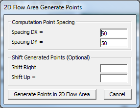
Figure 5 43. 2D Flow Area Computational Point Spacing Editor
After the Computational Point Spacing (DX and DY) has been entered, press the Generate Points in 2D flow area button. Pressing this button will cause the software to compute a series of X and Y coordinates for the cell centers. The user can view these points by pressing the View/Edit Computational Point's button, which brings the points up in a table. The user can cut and paste these into a spreadsheet, or edit them directly if desired (It is not envisioned that anyone will edit the points in this table or Excel, but the option is available).
There are five additional fields on the 2D Flow Areas editor (Figure 5-42) that are used during the 2D pre-processing. These fields are:
Default Manning's n Value: This field is used to enter a default Manning's n values that will be used for the Cell Faces in the 2D Flow Area. User's have the option of adding a spatially varying landuse classification versus Manning's n value table (and a corresponding Land Classification layer in RAS-Mapper), which can be used to override the base Manning's n values where polygons and roughness are defined. Even if a Land Use Classification versus Manning's n value table is defined, for any areas of the 2D Flow Area not covered by that layer, the base/default Manning's n value will be used for that portion of the 2D Flow Area.
Cell Volume Filter Tol: This tolerance is used to reduce the number of points in the 2D cell elevation volume curves that get developed in the 2D Pre-processor. Fewer points in the curve will speed up the computations, but reduce the accuracy of the elevation volume relationship. The default tolerance for filtering these points is 0.01 ft.
Face Profile Filter Tol: This filter tolerance is used to reduce the number of points that get extracted from the detailed terrain for each face of a 2D cell. The default is 0.01 ft.
Face Area-Elev Filter Tol: This filter tolerance is used to reduce the number of points in the cell face hydraulic property tables. Fewer points in the curves will speed up the computations, but reduce the accuracy of the face hydraulic property relationships. The default is 0.01 ft.
Face Conveyance Tol Ratio:This tolerance is used to figure out if more or less points are required at the lower end of the face property tables. It first computes conveyance at all of the elevations in the face property tables. It then computes the conveyance at an elevation half way between the points and compares this value to that obtained by using linear interpolation (based on the original points). If the computed value produces a conveyance that is within 2% (0.02) of the linear interpolation value, then no further points are needed between those two values. If linear interpolation would produce a value of conveyance that is more than 2% from the computed value at that elevation, then a new point is added to that table. This reduces the error in computing hydraulic properties, and therefore conveyance due to linear interpolation of the curves. A higher tolerance will results in fewer points in the hydraulic property tables of the cell faces, but less hydraulic accuracy for the flow movement across the faces. The default value is 0.02, which represents a 2% change.
Face Laminar Depth: This field is used to define the depth of water at which turbulent flow would transition to laminar flow for sheet flow flowing over a plane. The default is 0.2 feet.
Once a nominal grid size has been selected and a base Manning's n-value has been entered, the user should press the OK button to accept the data and close the editor. When the OK button is selected the software automatically creates the computational mesh and displays it in the Geometric Data Editor graphics window (See Figure 5-44).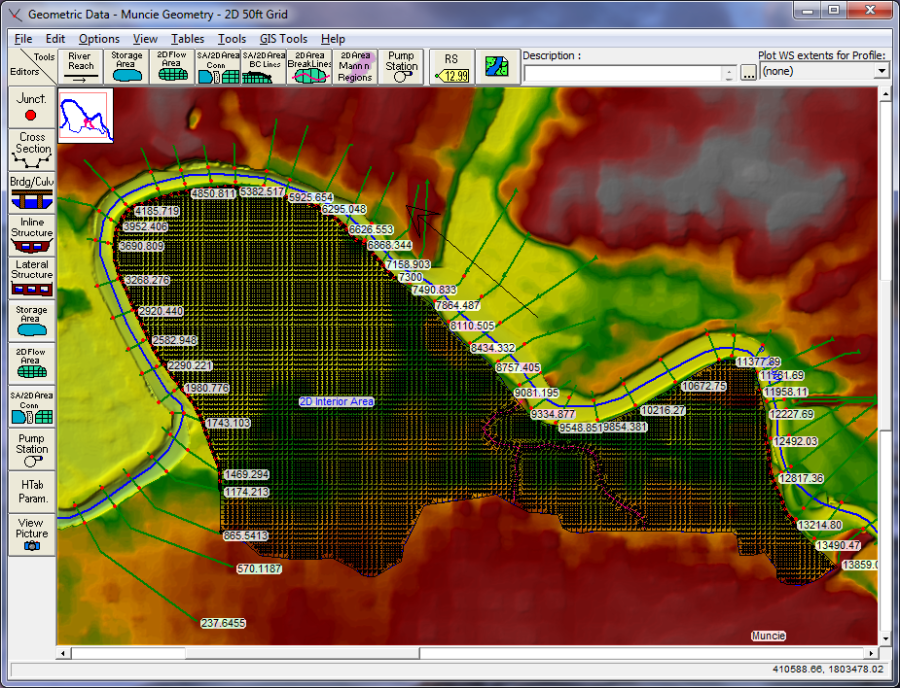
Figure 5 44. Example 2D computational mesh for an interior of a levee protected area.
As mentioned previously, cells around the 2D Flow Area boundary will be irregular in shape, in order to conform to the user entered polygon. The mesh generation tools utilize the irregular boundary, as well as try to ensure that no cell is smaller in area than the nominal cell size. The cells around the boundary will be equal to or larger than the nominal cell size; therefore, if a boundary cell is going to be smaller than the nominal cell size it gets combined with a neighbor cell. Additionally, breaklines can be placed inside of a 2D Flow Area in order to align the mesh to a geometric feature (levee, road, etc…) Shown in Figure 5-45, is a zoomed in view of a mesh with break lines on top of levees. 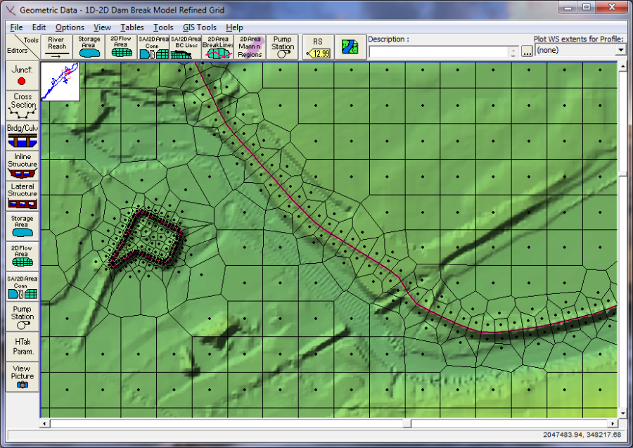
Figure 5 45. Zoomed in view of the 2D Flow Area computational mesh.
The HEC-RAS terminology for describing the computational mesh for 2D modeling begins with the 2D Flow Area. The 2D Flow Area defines the boundary for which 2D computations will occur. A computational mesh (or computational grid) is created within the 2D Flow Area.
Each cell within the computational mesh has the following three properties:
Cell Center:The computational center of the cell. This is where the water surface is computed for the cell.
Cell Faces:These are the cell boundary faces. Faces are generally straight lines, except along the outer boundary of the 2D Flow Area, in which a cell face can be a multi-point line.
Cell Face Points:The cell Face Points (FP) are the ends of the cell faces. Later on in this document the Face Point (FP) numbers for the outer boundary of the 2D Flow Area will be used to hook the 2D Flow Area to a Lateral Structure.
Figure 5 46. Description of HEC-RAS 2D modeling computational mesh terminology.
Edit/Modify the Computational Mesh
The computational mesh will control the movement of water through the 2D flow area. Specifically, one water surface elevation is calculated for each grid cell center at each time step. The computational cell faces control the flow movement from cell to cell. Within HEC-RAS, the underlying terrain and the computational mesh are preprocessed in order to develop detailed elevation–volume relationships for each cell, and also detailed hydraulic property curves for each cell face (elevation vs. wetted perimeter, area, and roughness). By creating hydraulic parameter tables from the underlying terrain, the net effect is that the details of the underlying terrain are still taken into account in the water storage and conveyance, regardless of the computational cell size. However, there are still limits to what cell size should be used, and important considerations for where smaller detailed cells are needed versus larger coarser cells.
In general, the cell size should be based on the slope of the water surface in a given area, as well as barriers to flow within the terrain. Where the water surface slope is flat and not changing rapidly, larger grid cell sizes are appropriate. Steeper slopes, and localized areas where the water surface elevation and slope change more rapidly will require smaller grid cells to capture those changes. Since flow movement is controlled by the computational cell faces, smaller cells may be required to define significant changes to geometry and rapid changes in flow dynamics.
The computational mesh can be edited/modified with the following tools: break lines; moving points; adding points, and removing points.
Break Lines
The user can add new break lines at any time. HEC-RAS allows the user to enter a new break line on top of an existing mesh and then regenerate the mesh around that break line, without changing the computational points of the mesh in other areas. The user can draw a new break line, then left click on the break line and select the option Enforce Break line in 2D Flow Area. Once this option is selected, new cells will be generated around the break line with cell faces that are aligned along the break line. Any existing cell centers that were already in the mesh in the area of the break line are remove first (within a buffer zone around the break line, based on the cell size used around the break line).
Additionally the user can control the size/spacing of cells along the break line. To control the cell spacing along a break line, right click on the break line and select the option Edit Break Line Cell Spacing. A window will appear allowing the user to enter a minimum and maximum cell spacing to be used when forming cells along that break line. The minimum cell spacing is used directly along the break line. The software will then increase the cell size around the break line, in order to provide a gradual cell size transition from the break line to the nominal cell size being used for the mesh. The user can enter a Maximum cell size if desired. If no maximum cell size is entered, the software automatically transitions the cells from the minimum cell size around the break line, to the default mesh cell size. To enforce the new cell spacing, the user must select the Enforce Break line in 2D Flow Area option, after entering the break line cell spacing. Break line cell spacing's are saved, such that if the mesh is regenerated, the user defined break line cell spacing will automatically be used. User can also bring up a table that will show all of the break lines and any user entered break line cell spacing values. To open this table, select GIS Tools, then Break Lines Cell Spacing Table. Once the table is open, users can add or change break line cell spacing values from the table. Then if the user regenerates the whole mesh, or just the area around a specific break lines, the new break line cell spacing will be used.
When creating a mesh around a break line, it may be desirable or even necessary to use smaller cells than the nominal cell size used in other areas of the mesh. However, transitions from a larger cell size immediately to a smaller cell size, may not produce the most accurate computational model. So it is better to transition cell sizes gradually. The HEC-RAS mesh generation tools allow the user to enter a minimum and a maximum cell spacing to use around break lines. The mesh generation tools will automatically transition from the smaller cell size right at the break line to the larger cell size away from the break line.
Hand Based Mesh Editing Tools
The hand editing mesh manipulation tools are available under the Edit menu of the HEC-RAS Geometric Data editor. If the user selects Edit then Move Points/Object, the user can select and move any cell center or points in the bounding polygon. If a cell center is moved, all of the neighboring cells will automatically change due to this movement. If the user selects Edit then Add Points, then wherever the user left-clicks within the 2D flow area, a new cell center is added, and the neighboring cells are changed (once the mesh is updated). The software creates a local mesh (Just the area visible on the screen, plus a buffer zone), such that while you are editing, just the local mesh will get updated. The entire mesh only updates once the user has turned off the editing feature, which saves computational time in creating the new mesh. If the user selects Edit then Remove Points, then any click near a cell center will remove that cell's point, and all the neighboring cells will become larger to account for the removed cell.
The user may want to add points and move points in areas where more detail is needed. The user may also want to remove points in areas where less detail is needed. Because cells and cell faces are preprocessed into detailed hydraulic property tables, they represent the full details of the underlying terrain. In general, the user should be able to use larger grid cell sizes than what would be possible with a model that does not preprocess the cells and the cell faces using the underlying terrain. Many 2D models simply use a single flat elevation for the entire cell, and a single flat elevation for each cell face. These types of 2D models generally require very small computational cell sizes in order to model the details of the terrain.
HEC-RAS makes the computational mesh by following the Delaunay Triangulation technique and then constructing a Voronoi diagram (see Figure 5-47 below, taken from the Wikimedia Commons, a freely licensed media file repository):
Figure 5 47. Delaunay - Voronoi diagram example.
The triangles (black) shown in Figure 18 are made by using the Delaunay Triangulation technique (http://en.wikipedia.org/wiki/Delaunay_triangulation![]() ). The cells (red) are then made by bisecting all of the triangle edges (Black edges), and then connecting the intersection of the red lines (Voronoi Diagram). This is analogous to the Thiessen Polygon method for attributing basin area to a specific rain gage.
). The cells (red) are then made by bisecting all of the triangle edges (Black edges), and then connecting the intersection of the red lines (Voronoi Diagram). This is analogous to the Thiessen Polygon method for attributing basin area to a specific rain gage.
You may want to add points and move points in areas where you need more detail. You may also want to remove points in areas where you know you need less detail. Because cells and cell faces are pre-processed into detailed hydraulic property tables, they represent the full details of the underlying terrain. In general, you should be able to get away with larger grid cell sizes than what you would be able to with a model that does not do this pre-processing of the cells and the cell faces using the underlying terrain. Many 2D models simply use a single flat elevation for the entire cell, and a single flat elevation for each cell face. These types of 2D models generally require very small computational cell sizes in order to model the details of the terrain.