Download PDF
Download page Entering Bridge Scour Data.
Entering Bridge Scour Data
The bridge scour computations are performed by opening the Hydraulic Design Functions window and selecting the Scour at Bridges function. Once this option is selected the program will automatically go to the output file and get the computed output for the approach section, the section just upstream of the bridge, and the sections inside of the bridge. The Hydraulic Design window for Scour at Bridges will appear as shown in Figure 11-1.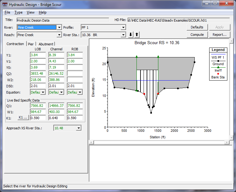
Figure 11 1. Hydraulic Design Window for Scour at Bridges
As shown in Figure 11-1, the Scour at Bridges window contains the input data, a graphic, and a window for summary results. Input data tabs are available for contraction scour, pier scour, and abutment scour. The user is required to enter only a minimal amount of input and the computations can be performed. If the user does not agree with any of the data that the program has selected from the output file, the user can override it by entering their own values. This provides maximum flexibility in using the software.
Entering Contraction Scour Data
Contraction scour can be computed in HEC-RAS by either Laursen's clear-water (Laursen, 1963) or live-bed (Laursen, 1960) contraction scour equations. Figure 11-2 shows all of the data for the contraction scour computations. All of the variables except K1 and D50 are obtained automatically from the HEC-RAS output file. The user can change any variable to whatever value they think is appropriate. To compute contraction scour, the user is only required to enter the D50 (mean size fraction of the bed material) and a water temperature to compute the K1 factor. 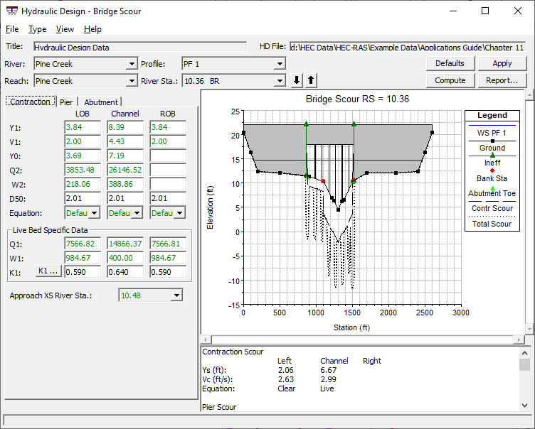
Figure 11 2. Example Contraction Scour Calculation
Each of the variables that are used in the computation of contraction scour are defined below, as well as a description of where each variable is obtained from the output file.
Y1: The average depth (hydraulic depth) in the left overbank, main channel, and the right overbank, at the approach cross-section.
V1: The average velocity of flow in the left overbank, main channel, and right overbank, at the approach section.
Y0: The average depth in the left overbank, main channel, and right overbank, at the contracted section. The contracted section is taken as the cross section inside the bridge at the upstream end of the bridge (section BU).
Q2: The flow in the left overbank, main channel, and right overbank, at the contracted section (section BU).
W2: The top width of the active flow area (not including ineffective flow area), taken at the contracted section (section BU).
D50: The bed material particle size of which 50% are smaller, for the left overbank, main channel, and the right overbank. These particle sizes must be entered in millimeters by the user.
Equation: The user has the option to allow the program to decide whether to use the live-bed or clear-water contraction scour equations, or to select a specific equation. If the user selects the Default option (program selects which equation is most appropriate), the program must compute Vc, the critical velocity that will transport bed material finer than D50. If the average velocity at the approach cross section is greater than Vc, the program uses the live-bed contraction scour equation. Otherwise, the clear-water contraction scour equation will be used.
Q1: The flow in the left overbank, main channel, and right overbank at the approach cross-section.
W1: The top width of the active flow area (not including ineffective flow area), taken at the approach cross section.
K1: An exponent for the live-bed contraction scour equation that accounts for the mode of bed material transport. The program can compute a value for K1 or the user can enter one. To have the program compute a value, the K1 button must be pressed. Figure 11-3 shows the window that comes up when the K1 button is pressed. Once a water temperature is entered, and the user presses the OK button, the K1 factor will be displayed on the main contraction scour window. K1 is a function of the energy slope (S1) at the approach section, the shear velocity (V* ) at the approach section, water temperature, and the fall velocity (w) of the D50 bed material.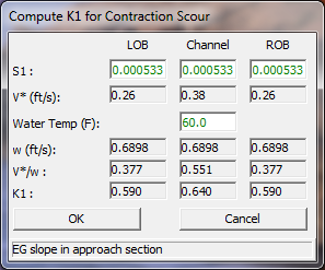
Figure 11 3. Computation of the K1 Factor
Approach XS River Sta.: The river station of what is being used as the approach cross section. The approach cross section should be located at a point upstream of the bridge just before the flow begins to contract do to the constriction of the bridge opening. The program assumes that the second cross section upstream of the bridge is the approach cross section. If this is not the case, the user can select a different river station to be used as the approach cross section.
As shown in Figure 11-2, the computation of contraction scour is performed separately for the left overbank, main channel, and right overbank. For this example, since there is no right overbank flow inside of the bridge, there is no contraction scour for the right overbank. The summary results show that the computed contraction scour, Ys, was 2.06 feet for the left overbank, and 6.67 feet for the main channel. Also note that the graphic was updated to show how far the bed would be scoured due to the contraction scour.
Entering Pier Scour Data
Pier scour can be computed by either the Colorado State University (CSU) equation (Richardson, et al, 1990) or the Froehlich (1988) equation (the Froehlich equation is not included in the HEC No.18 report). The CSU equation is the default. As shown in Figure 11-4, the user is only required to enter the pier nose shape (K1), the angle of attack for flow hitting the piers, the condition of the bed (K3), and a D95 size fraction for the bed material. All other values are automatically obtained from the HEC-RAS output file.
As shown in Figure 11 4, the user has the option to use the maximum velocity and depth in the main channel, or the local velocity and depth at each pier for the calculation of the pier scour. In general, the maximum velocity and depth are used in order to account for the potential of the main channel thalweg to migrate back and forth within the bridge opening. The migration of the main channel thalweg could cause the maximum potential scour to occur at any one of the bridge piers.
Each of the variables that are used in the computation of pier scour are defined below, as well as a description of where each variable is obtained from the output file.
Maximum V1 Y1: If the user selects this option, the program will find the maximum velocity and depth located in the cross section just upstream and outside of the bridge. The program uses the flow distribution output to obtain these values. The maximum V1 and Y1 will then be used for all of the piers.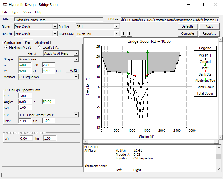
Figure 11 4. Example Pier Scour Computation
Local V1 Y1: If the user selects this option, the program will find the velocity (V1) and depth (Y1) at the cross section just upstream and outside of the bridge that corresponds to the centerline stationing of each of the piers.
Method: The method option allows the user to choose between the CSU equation and the Froehlich equation for the computation of local scour at bridge piers. The CSU equation is the default method.
Pier #: This selection box controls how the data can be entered. When the option "Apply to All Piers" is selected, any of the pier data entered by the user will be applied to all of the piers. The user does not have to enter all of the data in this mode, only the portion of the data that should be applied to all of the piers. Optionally, the user can select a specific pier from this selection box. When a specific pier is selected, any data that has already been entered, or is applicable to that pier, will show up in each of the data fields. The user can then enter any missing information for that pier, or change any data that was already set.
Shape: This selection box is used to establish the pier nose (upstream end) shape. The user can select between square nose, round nose, circular cylinder, group of cylinders, or sharp nose (triangular) pier shapes. When the user selects a shape, the K1 factor for the CSU equation and the Phi factor for the Froehlich equation are automatically set. The user can set the pier nose shape for all piers, or a different shape can be entered for each pier.
a: This field is used to enter the width of the pier. The program automatically puts a value in this field based on the bridge input data. The user can change the value.
D50: Median diameter of the bed material of which 50 percent are smaller. This value is automatically filled in for each pier, based on what was entered for the left overbank, main channel, and right overbank, under the contraction scour data. The user can change the value for all piers or any individual pier. This value must be entered in millimeters.
Y1: This field is used to display the depth of water just upstream of each pier. The value is taken from the flow distribution output at the cross section just upstream and outside of the bridge. If the user has selected to use the maximum Y1 and V1 for the pier scour calculations, then this field will show the maximum depth of water in the cross section for each pier. The user can change this value directly for each or all piers.
V1: This field is used to display the average velocity just upstream of each individual pier. The value is taken from the flow distribution output at the cross section just upstream and outside of the bridge. If the user has selected to use the maximum Y1 and V1 for the pier scour calculations, then this field will show the maximum velocity of water in the cross section for all piers. The user can change this value directly for each or all piers.
Angle: This field is used to enter the angle of attack of the flow approaching the pier. If the flow direction upstream of the pier is perpendicular to the pier nose, then the angle would be entered as zero. If the flow is approaching the pier nose at an angle, then that angle should be entered as a positive value in degrees. When an angle is entered, the program automatically sets a value for the K2 coefficient. When the angle is > 5 degrees, K1 is set to 1.0.
L: This field represents the length of the pier through the bridge. The field is automatically set by the program to equal the width of the bridge. The user can change the length for all piers or each individual pier. This length is used in determining the magnitude of the K2 factor.
K1: Correction factor for pier nose shape, used in the CSU equation. This factor is automatically set when the user selects a pier nose shape. The user can override the selected value and enter their own value.
K2: Correction factor for angle of attack of the flow on the pier, used in the CSU equation. This factor is automatically calculated once the user enters the pier width (a), the pier length (L), and the angle of attack (angle).
K3: Correction factor for bed condition, used in the CSU equation. The user can select from: clear-water scour; plane bed and antidune flow; small dunes; medium dunes; and large dunes.
D95: The median size of the bed material of which 95 percent is finer. The D95 size fraction is used in the computation of the K4 factor, and must be entered in millimeters directly by the user.
K4: The K4 factor is used to decrease scour depths in order to account for armoring of the scour hole. This factor is only applied when the D50 of the bed material is greater than 0.006 feet (0.2 mm) and the D95 is greater than 0.06 feet (2.0 mm). This factor is automatically calculated by the program, and is a function of D50; D95; a; and the depth of water just upstream of the pier. The K4 factor is used in the CSU equation.
a: The projected pier width with respect to the direction of the flow. This factor should be calculated by the user and is based on the pier width, shape, angle, and length. This factor is specific to Froehlich's equation.
Phi: Correction factor for pier nose shape, used in the Froehlich equation. This factor is automatically set when the user selects a pier nose shape. The user can override the selected value and enter their own value.
For the example shown in Figure 11 4 the CSU equation was used, resulting in a computed pier scour of 10.61 feet at each pier (shown under summary results in Figure 11 4). Also shown in Figure 11 4 is an updated graphic with both contraction and pier scour shown.
Entering Abutment Scour Data
Abutment scour can be computed by either the HIRE equation (Richardson, 1990) or Froehlich's equation (Froehlich, 1989). The input data and results for abutment scour computations are shown in Figure 11-5.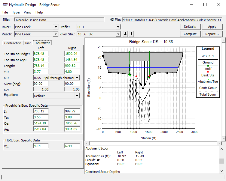
Figure 11 5. Example Abutment Scour Computations
As shown in Figure 11-5, abutment scour is computed separately for the left and right abutment. The user is only required to enter the abutment type (spill-through, vertical, vertical with wing walls). The program automatically selects values for all of the other variables based on the hydraulic output and default settings. However, the user can change any variable. The location of the toe of the abutment is based on where the roadway embankment intersects the natural ground. This stationing is very important because the hydraulic variables used in the abutment scour computations will be obtained from the flow distribution output at this cross section stationing. If the user does not like the stationing that the model picks, they can override it by entering their own value.
Each of the variables that are used in the computation of abutment scour are defined below, as well as a description of where each variable is obtained from the output file.
Toe Sta at Bridge: This field is used to define the stationing in the upstream bridge cross section (section BU), where the toe of the abutment intersects the natural ground. The program automatically selects a value for this stationing at the point where the road embankment and/or abutment data intersects the natural ground cross-section data. The location for the abutment toe stationing can be changed directly in this field.
Toe Sta at App.: This field is used to define the stationing in the approach cross section (section 4), based on projecting the abutment toe station onto the approach cross section. The location for this stationing can be changed directly in this field.
Length: Length of the abutment and road embankment that is obstructing the flow. The program automatically computes this value for both the left and right embankments. The left embankment length is computed as the stationing of the left abutment toe (projected up to the approach cross section) minus the station of the left extent of the active water surface in the approach cross section. The right embankment length is computed as the stationing of the right extent of the active water surface minus the stationing of the toe of the right abutment (projected up to the approach cross section), at the approach cross section. These lengths can be changed directly.
Y1: This value is the computed depth of water at the station of the toe of the embankment, at the cross section just upstream of the bridge. The value is computed by the program as the elevation of the water surface minus the elevation of the ground at the abutment toe stationing. This value can also be changed by the user. This value is used in the HIRE equation.
K1: This value represents a correction factor accounting for abutment shape. The user can choose among: vertical abutments; vertical with wing walls; and spill-through abutments.
Skew: This field is used to enter the angle of attack of the flow against the abutment. A value of 90 degrees should be entered for abutments that are perpendicular to the flow (normal situation). A value less than 90 degrees should be entered if the abutment is pointing in the downstream direction. A value greater than 90 degrees should be entered if the abutments are pointing in the upstream direction. The skew angle is used in computing the K2 factor.
K2: Correction factor for angle of attack of the flow on the abutments. This factor is automatically computed by the program. As the skew angle becomes greater than 90 degrees, this factor increases from a value of one. As the skew angle becomes less than 90 degrees, this value becomes less than one.
Equation: This field allows the user to select a specific equation (either the HIRE or Froehlich equation), or select the default mode. When the default mode is selected, the program will choose the equation that is the most applicable to the situation. The selection is based on computing a factor of the embankment length divided by the approach depth. If this factor is greater than 25, the program will automatically use the HIRE equation. If the factor is equal to or less than 25, the program will automatically use the Froehlich equation.
L': The length of the abutment (embankment) projected normal to the flow (projected up to the approach cross section). This value is automatically computed by the program once the user enters an abutment length and a skew angle. This value can be changed by the user.
Ya: The average depth of flow (hydraulic depth) that is blocked by the embankment at the approach cross section. This value is computed by projecting the stationing of the abutment toe's up to the approach cross section. From the flow distribution output, the program calculates the area and top width left of the left abutment toe and right of the right abutment toe. Ya is then computed as the area divided by the top width. This value can be changed by the user directly.
Qe: The flow obstructed by the abutment and embankment at the approach cross section. This value is computed by projecting the stationing of the abutment toes onto the approach cross-section. From the flow distribution output, the program calculates the percentage of flow left of the left abutment toe and right of the right abutment toe. These percentages are multiplied by the total flow to obtain the discharge blocked by each embankment. These values can be changed by the user directly.
Ae: The flow area that is obstructed by the abutment and embankment at the approach cross section. This value is computed by projecting the stationing of the abutment toes onto the approach cross-section. From the flow distribution output, the program calculates the area left of the left abutment toe and right of the right abutment toe. These values can be changed by the user directly.
V1: The velocity at the toe of the abutment, taken from the cross section just upstream and outside of the bridge. This velocity is obtained by finding the velocity in the flow distribution output at the corresponding cross section stationing of the abutment toe. These values can be changed by the user directly.
In addition to the abutment input data, once the compute button is pressed, the bridge scour graphic is updated to include the abutment scour and the summary results window displays the computed abutment results. For the example shown in Figure 11-5, the program selected the HIRE equation and computed 10.92 feet of local scour for the left abutment and 15.49 feet of local scour for the right abutment.
Computing Total Bridge Scour
The total scour is a combination of the contraction scour and the individual pier and abutment scour at each location. Table 12.1 shows a summary of the computed results, including the total scour.
Table 12.1
Summary of Scour Computations
Contraction Scour
Left O.B. Main Channel Right O.B.
Ys =2.06 ft (0.63 m)6.67 ft (2.03 m)0.00 ft (0.0 m)
Eqn =Clear-Water Live-Bed
Pier Scour
Piers 1-6 Ys = 10.61 ft (3.23 m)
Eqn. =CSU equation
Abutment Scour
Left Right
Ys =10.92 ft (3.33 m)15.49 ft (4.72 m)
Eqn =HIRE equation HIRE equation
Total Scour
Left Abutment =12.98 ft (3.96 m)
Right abutment =22.16 ft (6.76 m)
Piers 1-2 (left O.B.)=12.67 ft (3.86 m)
Piers 3-6 (main ch.)=17.28 ft (5.27 m)
Once all three types of scour data are entered, and the compute button is pressed, the bridge scour graphic is updated to reflect the total computed scour. Shown in Figure 11-6 is the graphic of the final results (the graphic has been zoomed in to see more detail). The graphic and the tabular results can be sent directly to the default printer, or they can be sent to the Windows Clipboard in order to be pasted into a report. A detailed report can be generated, which shows all of the input data, computations, and final results.
The bridge scour input data can be saved by selecting Save Hydraulic Design Data As from the File menu of the Hydraulic Design Function window. The user is only required to enter a title for the data. The computed bridge scour results are never saved to the hard disk. The computations can be performed in a fraction of a second by simply pressing the compute button. Therefore, when the Hydraulic Design Function window is closed, and later re-opened, the user must press the compute button to get the results.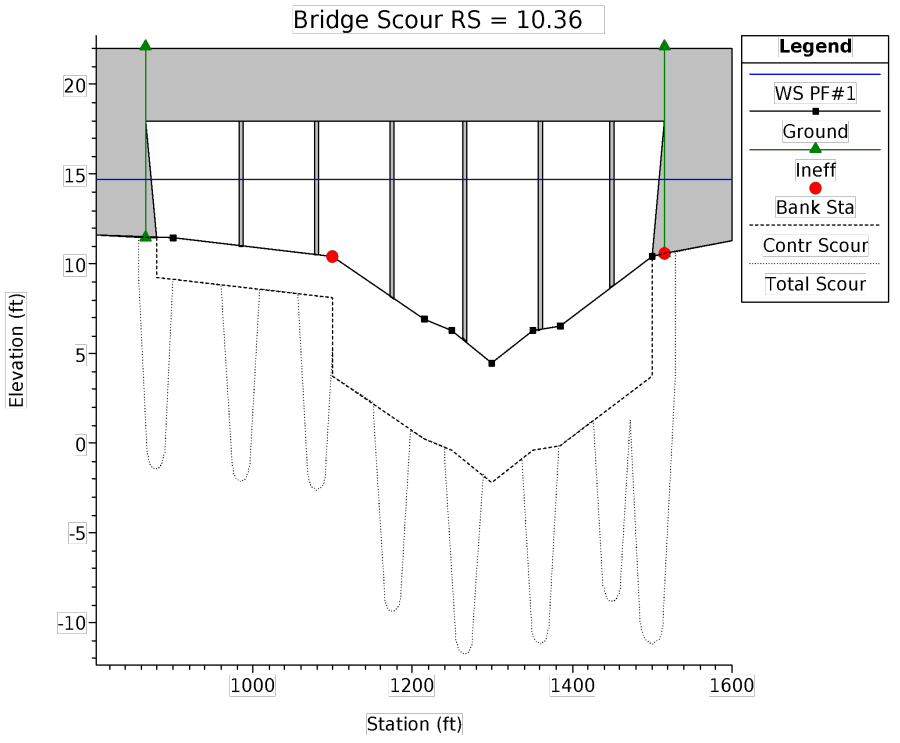
Figure 11 6. Total Scour Depicted in Graphical Form