Download PDF
Download page Piecewise Linear Regression.
Piecewise Linear Regression
Often, a single power function does not capture the complexity of the data. Sediment data tend to over-represent low flows, which can dominate the regression in the moderate-to-large flow range that is most morphologically active. Additionally, "bent" or "inflected" rating curves are relatively common, particularly in supply limited systems. Future version of this tool will include local regression methods, that will allow users to develop more sophisticated rating curves. But a two-slope, piece-wise linear, regression can capture some of this complexity. HEC worked with UC Davis () to develop a piecewise linear algorithm that identifies the inflection point in an inflected or bent rating curve and fits a continuous model to the upper and lower halves of the data.
Piecewise Regression Approach
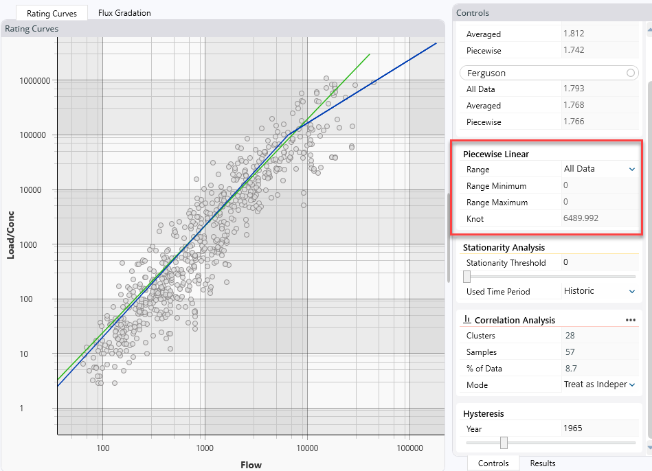
The simplest form of the piecewise linear model is included in the figure above. Change the Range from None to All Data. The calculator evaluates every data point as a potential inflection point (i.e. "knot" in the statistical terminology) and fits separate-but-continuous power functions to the upstream and downstream data. The algorithm selects the inflection point with the lowest Root Mean Square Error (RMSE). In the case pictured above, the model computed an inflection point at 6,490 cfs, and fit a steeper slope to the lower flows than the higher flows (which is typical of rivers in this region). Because most of the sediment moves in the moderate-to-large flow range, fitting a separate slope to these larger flows can affect the sediment budget and model dramatically.
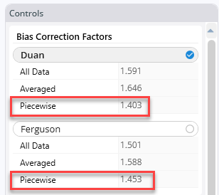
The piecewise linear model also computes biased and unbiased regressions. If you select this option, it will update the Piecewise correction factors for both Duan and Furguson (below) and will plot and report the unbiased result by default. Users can request the biased result, but this is not recommended.
Constraining the Inflection Point Range
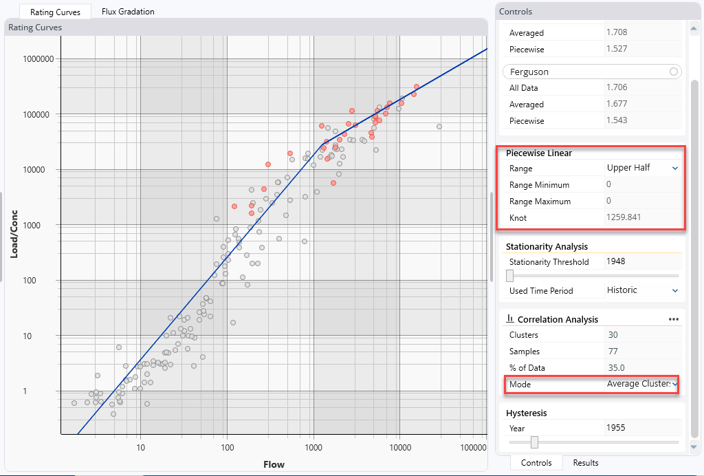
Because sediment data often over-represent the low flows, the flow-load inflection point that minimizes the RMSE can turn up in the lower flows (see Figure below). But because these flows do not deliver much sediment, the total sediment load will not be very sensitive to this constraint.
In some cases, the data can have multiple, local, minimums, in the RMSE, including a potential inflection point in the higher flow data that is not the global RMSE minimum. For example, the following figure includes the RMSE computed from each candidate inflection point. The global minimum is associated with a low flow, but there is a much higher flow inflection point that improves the overall fit substantially.
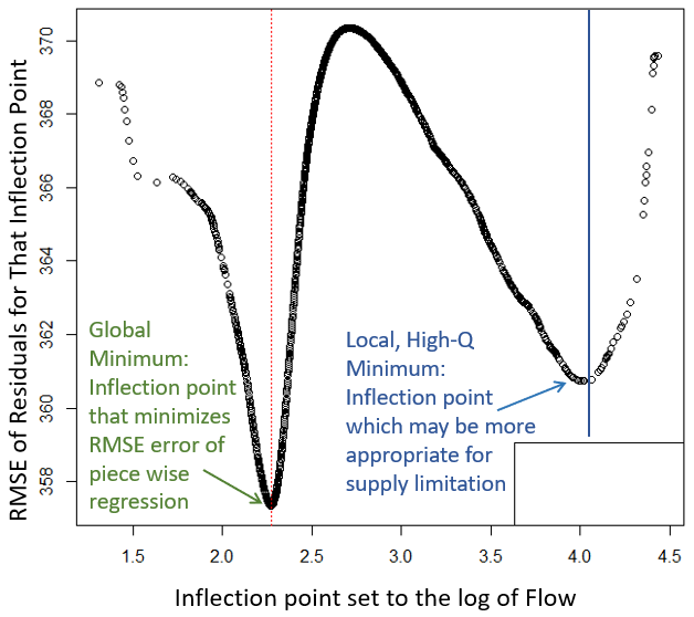
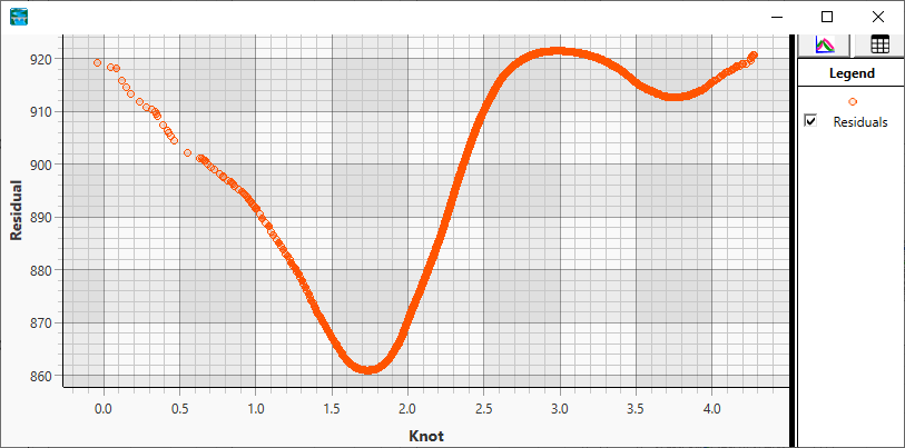
In versions 6.4 and later, you can plot these residuals by pressing the View Computed Residuals button. ![]()
By constraining the inflection-point candidates to a particular flow range, users can force the model to select a local minimum and specify an inflection point that is more morphologically meaningful.
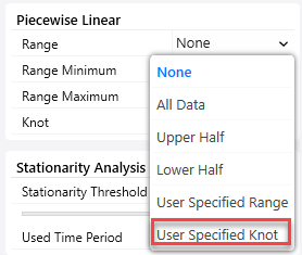
The tool includes three options to constrain the search range:
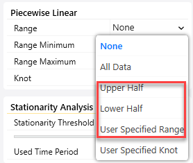
The Upper Half and Lower Half methods split the data and search the specified half for a local minimum, or users can specify a range over which the algorithm will search for a minimum.
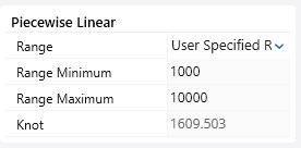
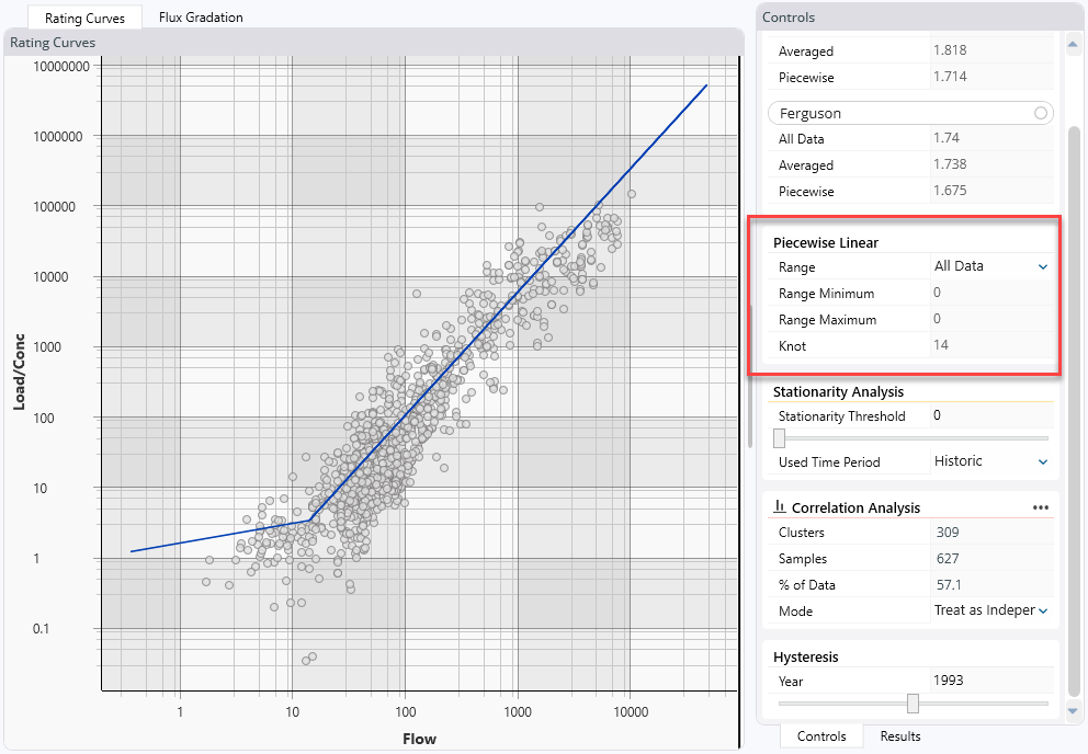
The following figure fits a piecewise linear model to the same data that set the inflection point at 14cfs above, but searches for an inflection point above 1,000 cfs. The rating curve below the inflection point is very similar to the simple power function, but the piecewise linear model fits those higher flows better.
Do Not Use Inflection Points on the Edge of the Range
Be careful of inflection points on the edge of the range. If you constrain the range to half the data, and the algorithm computes the median flow as the inflection point, it did not find a local minimum in the specified half of the data. Both the local and global minimum are outside the range, and a larger range should be used. This is also the case if the inflection point corresponds to either end of the user-specified range.
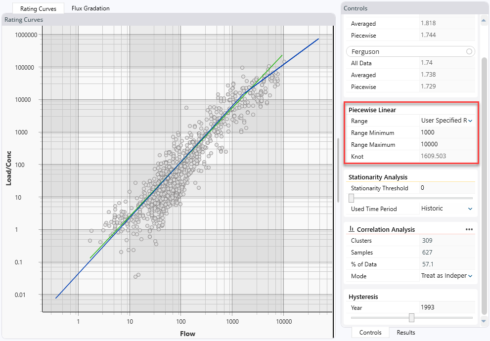
Finally, if the analyst has a physical justification for specifying an inflection point at a particular flow, the tool includes a User Specified option. In this option, the algorithm will assume the specified inflection point and minimize the slopes above and below it for the lowest error regression.
Use Temporal Averaging with Piecewise Linear Regression
Like all of the statistical tools, the piecewise linear model assumes data points are independent. Analyze the data for autocorrelation and apply any temporal averaging before selecting a final rating curve.