Calibration of Unsteady Flow Models

Calibration is the adjustment of a model's parameters, such as roughness and hydraulic structure coefficients, so that it reproduces observed data to an acceptable accuracy. The following is a list of common problems and factors to consider when calibrating an unsteady flow model.

Observed Hydrologic Data

Stage Records

In general, measured stage data is our most accurate hydrologic data. Measured stage data is normally well within +/- 1.0 feet of accuracy. However, errors can be found in measured stage data. Some common problems are:

1. The gages float gets stuck at a certain elevation during the rise or fall of the flood wave.
2. The recorder may systematically accumulate error over time.
3. The gage reader of a daily gage misses several days (cooperative stream gage program).
4. There is an error in the datum of the gage.
5. Subsidence over time causes errors in the stage measurement.

Flow Records

Flow records are generally computed from observed stages using single valued rating curves. These rating curves are a best fit of the measured data. The USGS classifies good flow measurements from Price current meters to be within ±5% of the true value. Some believe that this assumed error is optimistic. In any case, ±5% on many river systems, translates into a stage error of ±1.0 feet. Acoustic velocity meters (AVM) provide a continuous record, but the current USGS technique calibrates these meters to reproduce measurements from Price current meters, so the AVM is as accurate as the current meter. Boat measurements are almost always suspect. In general it is very difficult to get accurate velocity measurements using a price current meter from a boat. Newer techniques using acoustic velocity meters with three beams mounted on boats are thought to be much better.

Published discharge records should also be scrutinized. Continuous discharge is computed from discharge measurements, usually taken at bi-weekly or monthly intervals and the continuous stage record. The measurements are compiled into a rating curve and the departures of subsequent measurements from the rating curve are used to define shifts. The shifts are temporary changes in the rating curve due to unsteady flow effects (looped rating curve) and short term geomorphic changes. The quality of the record depends on the frequency of discharge measurements and the skill of the hydrologist. The only way to depict the quality of the published flow data is to compare the measured flow values to the currently published rating curve. However, if the flow measurements are infrequent, one can only apply the flow record to the model and see how well the stage record is reproduced. Remember! Most published flow records for large streams are in mean daily flow. The modeler must somehow assign time values to these records.

High Water Marks 

High water marks are estimated from the upper limit of stains and debris deposits found on buildings, bridges, trees, and other structures. Wind and wave actions can cause the debris lines to be higher than the actual water surface. Capillary action can cause stains on buildings to migrate upward, depending on the material used for the building walls. High water marks in the overbank area are often higher than in the channel. The overbank water is moving slower and may be closer to the energy gradeline. High water marks on bridge piers are often equal to the energy gradeline, not the average water surface. This is due to the fact that the water will run up the front of the pier to an elevation close to the energy gradeline. 

A comparison between high water marks and the computed maximum water surface profile is included in the figure below. Note the scatter in the high water marks, which mark is accurate?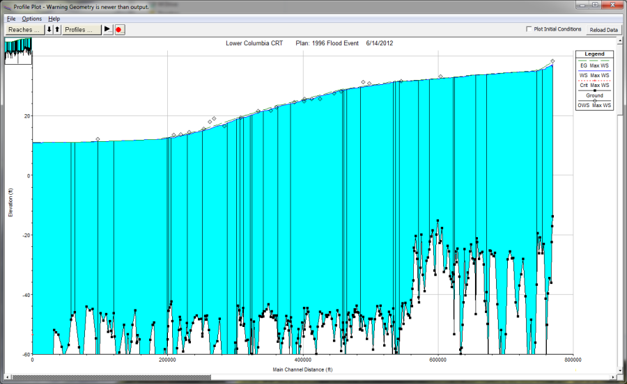 

Ungaged Drainage Area

For an unsteady flow model to be accurate, it must have flow input from all of the contributing area. In many studies a significant portion of the area is ungaged. Discharge from ungaged areas can be estimated from either hydrologic models or by taking flow from a gaged watershed with similar hydrologic characteristics and multiplying it by a simple drainage area ratio.

An example of accounting for ungaged drainage area is shown below for the Red River of the North.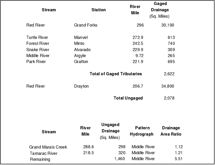

As shown in the above figure, ungaged areas can be accounted for by using a pattern hydrograph of a hydrologically similar watershed (Middle River), then calculating a drainage area ratio of contributing areas (Ungaged area divided by pattern hydrograph area).

River and Floodplain Geometry

It is essential to have an adequate number of cross sections that accurately depict the channel and overbank geometry. This can be a great source of error when trying to calibrate. Additionally, all hydraulic structures must be accurately depicted. Errors in bridge and culvert geometry can be significant sources of error in computed water surface profiles. Another important factor is correctly depicting the geometry at stream junctions (flow combining and splitting locations). This is especially important at flow splits, and areas in which flow reversals will occur (i.e. flow from a main stem backing up a tributary).

Also, a one-dimensional model assumes a constant water surface across each cross section. For some river systems, the water surface may vary substantially between the channel and the floodplain. If this is the case in your model, it may be necessary to separate the channel and the floodplain into their own reaches or model the overbank area as a series of storage areas.

Roughness Coefficients

Roughness coefficients are one of the main variables used in calibrating a hydraulic model. Generally, for a free flowing river, roughness decreases with increased stage and flow (Figure 7-31). However, if the banks of a river are rougher than the channel bottom (due to trees and brush), then the composite n value will increase with increased stage. Sediment and debris can also play an important role in changing the roughness. More sediment and debris in a river will require the modeler to use higher n values in order to match observed water surfaces.  An example plot of roughness versus discharge for the Mississippi River at Arkansas City is shown below.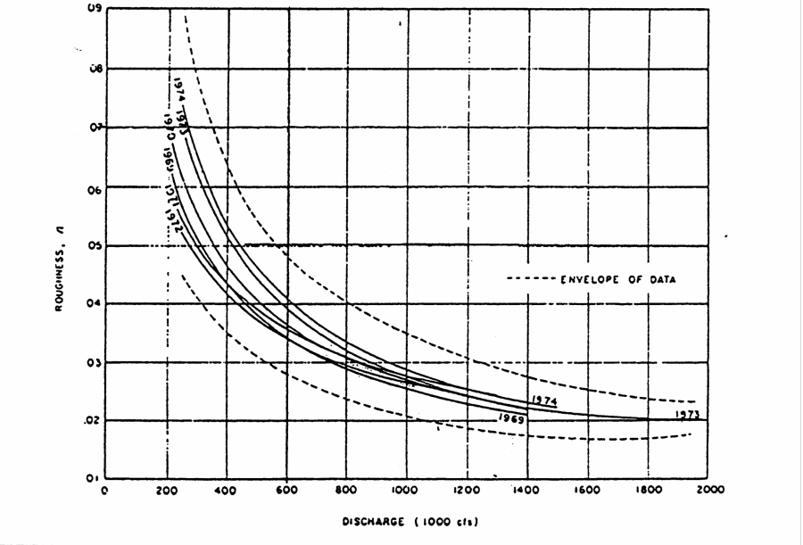

Looped Rating Curves

Excluding cataclysmic events such as meander cutoffs or a new channel, the river will pass any given flow within a range of stages. The shift in stage is a result of the following: shifts in channel geometry or bed forms; the dynamics of the hydrograph (how fast the flood wave rises and falls); backwater (backwater can significantly change the stage at a given cross section for a given flow); and finally, the slope of the river (flatter streams tend to have greater loops in the rating curve). The figure below shows a looped rating for a single event. Generally, the lower stages are associated with the rising side of a flood wave, and the higher stages are associated with the falling side of the flood wave.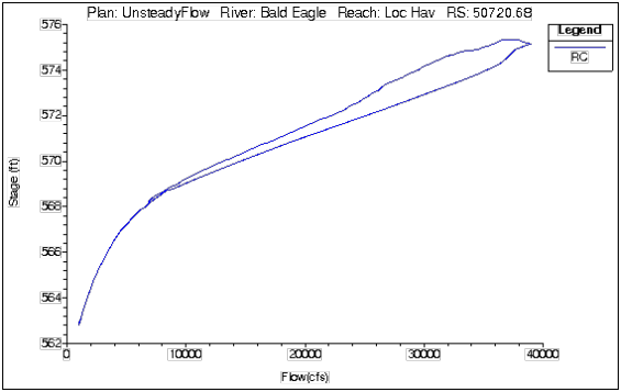

Alluvial Rivers

In an alluvial stream the channel boundary, as well as the meandering pattern of the stream, are continuously being re-worked by the flow of water. Alluvium is unconsolidated granular material, which is deposited by flowing water. An alluvial river is incised into these alluvial deposits. The flow characteristics of the stream are defined by the geometry and roughness of the cross-section below the water surface. The reworking of the cross section geometry and meander pattern is greatest during high flow, when the velocity, depth of water, and sediment transport capacity are the greatest. For some streams, which approach an equilibrium condition, the change in morphology (landforms) is small. For other streams, the change in morphology is much larger. The change can be manifest as changes in roughness or a more dynamic change such as the cut-off of a meander loop, which shortens the stream and starts a process which completely redefines the bed.

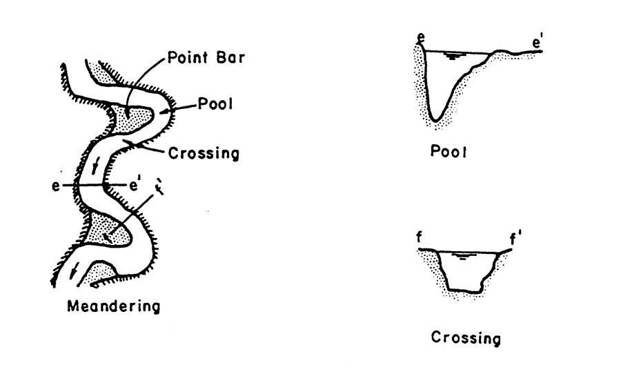
As shown in the figure below of a meandering river, pools are at the outside of bends, and a typical pool cross-section is very deep. On the inside of the bend is a point bar. Crossings are between the meander bends. A typical crossing cross-section is much shallower and more rectangular than a pool cross-section.  The morphology of a typical meandering river is shown below.

An invert profile for the Mississippi River is shown in the the figure below. Note the pools and crossings. The water surface profile is controlled by the crossing cross-sections (high points in the invert), particularly at low flow. The conveyance properties of pool cross-sections are only remotely related to the water surface. This poses a significant problem when calibrating a large river.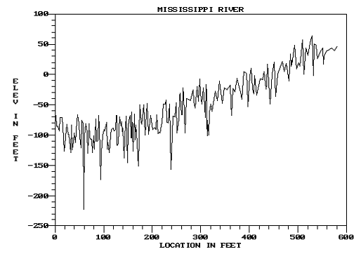

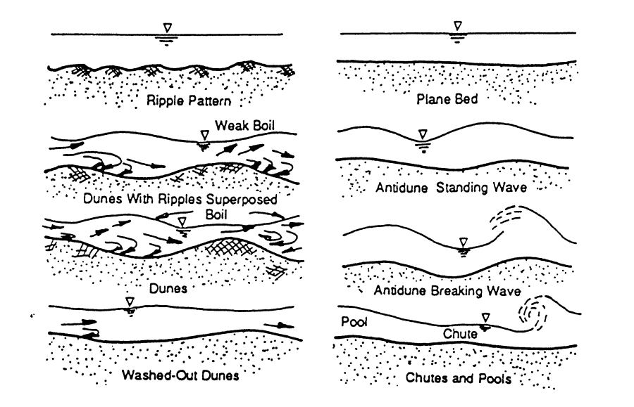
As stage and flow increase you have an increase in stream power (stream power is a function of hydraulic radius, slope, and velocity). The bed forms in an alluvial stream tend to go through the following transitions:

1. Plane bed without sediment movement.
2. Ripples.
3. Dunes.
4. Plane bed with sediment movement.
5. Anti-dunes.
6. Chutes and pools.

Generally, anti-dunes and chutes and pools are associated with high velocity streams approaching supercritical flow. The bed form process for alluvial streams is shown in the figure below.
 
Typical Manning's roughness coefficients for the different bed forms of alluvial streams presented above are shown in the table below.

Note: This table is from the book "Engineering Analysis of Fluvial Streams", by Simons, Li, and Associates.

Bed forms also change with water temperature. Because water is more viscous at lower temperatures, it becomes more erosive, reducing the height and the length of the dunes. At higher temperatures, when the water is less viscous, the dunes are higher and of greater length. Since the larger dunes are more resistant to flow, the same flow will pass at a higher stage in the summer than in the winter. Larger rivers such as the Mississippi River and the Missouri River show these trends. The figure below shows the seasonal shift in bed roughness due to water temperature for the Mississippi River at St. Louis.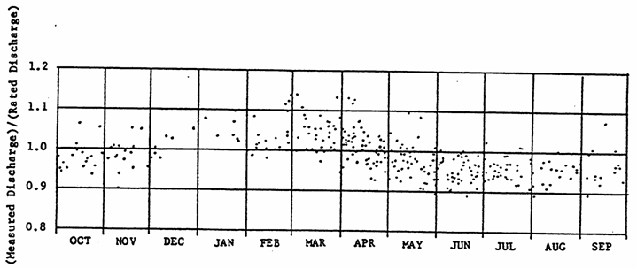 

River and Floodplain Storage

Cross Sectional Storage

The active flow area of a cross section is the region in which there is appreciable velocity. This part of the cross section is conveying flow in the downstream direction. Storage is the portion of the cross section in which there is water, but it has little or no velocity. Storage can be modeled within a cross section by using the ineffective flow area option in HEC-RAS. The water surface elevation within the cross section storage is assumed to have the same elevation as the active flow portion of the cross section. 

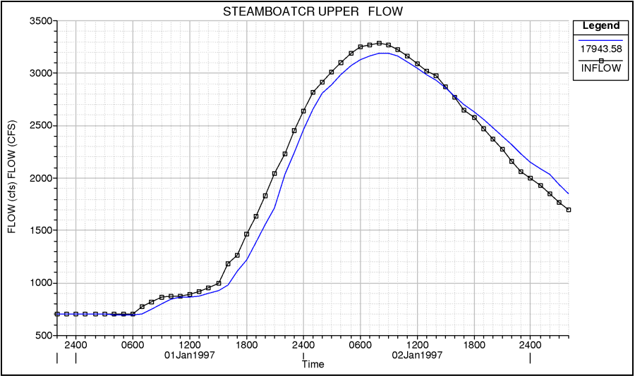
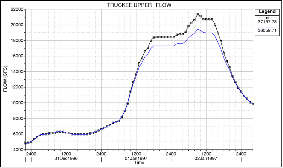
The storage within the floodplain is responsible for attenuating the flood hydrograph and, to some extent, delaying the flood wave. Effects of Overbank Storage. Water is taken out of the rising side of the flood wave and returned on the falling side. An example of the effects of overbank storage is shown in the figure below. In this example, the water goes out into storage during the rising side of the flood wave, as well as during the peak flow. After the peak flow passes, the water begins to come out of the storage in the overbank and increases the flow on the falling side of the floodwave.
 

Off Line Storage

Off line storage is an area away from the main river in which water can go from the main river to the ponding area. The connection between the ponding area and the river may be a designed overflow, or it may just be a natural overflow area. The water in the ponding area is often at a different elevation that the main river, therefore, it must be modeled separately from the cross sections describing the main river and floodplain. Within HEC-RAS, ponding areas are modeled using what we call a storage area. Storage areas can be connected hydraulically to the river system by using a lateral weir/spillway option in HEC-RAS.

The effect that off line storage has on the hydrograph depends on the available volume and the elevation at which flow can get into and out of the storage area. Shown in the figure below is an example of an off-line storage area that is connected to the river through a lateral weir/spillway. The flow upstream and downstream of the offline storage area remains the same until the water surface elevation gets higher than the lateral weir. Water goes out into the lateral storage facility the whole time it is above the weir (i.e. the storage area elevation is always lower than the river elevation in this example). This continues until later in the event, when the river elevation is below the lateral weir and flow can no longer leave the river. In this example, the flow in the storage area does not get back into the river system until much later in the event, and it is at a very slow rate (possible drained by culverts to a downstream location).

Hydraulic Structure Coefficients

Bridges and culverts tend to have a local effect on stage, and a minimum affect on the flow hydrograph (this depends on the amount of backwater they cause and the steepness of the stream). However, in flat streams, increases in a water surface at a structure can cause a backwater upstream for a substantial distance (depends on amount of stage increase and slope of the stream). The coefficients that are important in bridge modeling are: Manning's n values; contraction and expansion coefficients; pier loss coefficients, and pressure and weir flow coefficients for high flows. Culvert hydraulics are dependent upon the size of the culverts and shape of the entrance. Additional variables include Manning's n values and contraction and expansion coefficients.

The effects of Inline weirs/spillways can be substantial on both the stage and the flow attenuation of the hydrograph. The effects on the hydrograph will depend upon the available storage volume in the pool upstream of the structure, as well as how the structure is operated. Lateral weir/spillway structures can have a significant impact on the amount of water leaving the river system. Therefore gate and weir coefficients for these structures can be extremely critical to getting the right amount of flow leaving the system.

Tools Available in HEC-RAS to Support Model Calibration

The following is a list of tools that the user should be aware of and use frequently during any calibration of an HEC-RAS model:
1. Manning's n Value Tables (Tables for other parameters).
2. Flow versus Roughness Factors options.
3. Graphical Plots with Observed data options.

• Profile Plots
• Cross section Plot
• Hydrograph (Stage and Flow) Plots

4. Tabular Output Tables

Steps To Follow in the Calibration Process

The following is a general list of steps to follow when calibrating an unsteady flow model:

1. Run a range of discharges in the Steady-Flow mode (if possible), and calibrate n values to established rating curves at gages and known high water marks.
2. Select specific events to run in unsteady flow mode. Ensure each event encompasses the full range of flows from low to high and back to low flow.
3. Adjust cross section storage (ineffective areas) and lateral weirs to get good reproduction of flow hydrographs (Concentrate on timing, peak flow, volume, and shape).
4. Adjust Manning's n values to reproduce stage hydrographs.
5. Fine tune calibration for low to high stages by using "Discharge-Roughness Factors" where and when appropriate.
6. Further refine calibration for long-term modeling (period of record analysis) with "Seasonal Roughness Factors" where and when appropriate.
7. Verify the model calibration by running other flow events or long term periods that were not used in the calibration.
8. If further adjustment is deemed necessary from verification runs, make adjustments and re-run all events (calibration and verification events).

General Trends When Adjusting Model Parameters

n order to understand which direction to adjust model parameters to get the desired results, the following is a discussion of general trends that occur when specific variables are adjusted. These trends assume that all other geometric data and variables will be held constant, except the specific variable being discussed.
Impacts of Increasing Manning's n. When Manning's n is increased the following impacts will occur:

1. Stage will increase locally in the area where the Manning's n values were increased.
2. Peak discharge will decrease (attenuate) as the flood wave moves downstream.
3. The travel time will increase.
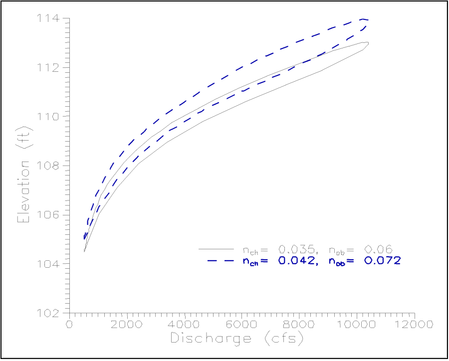
4. The loop effect will be wider (i.e. the difference in stage for the same flow on the rising side of the flood wave as the falling side will be greater). An example of this is looped curve is shown in the figure below.

Impacts of Increasing Storage. When storage within the floodplain is increased, the following impacts will occur:

1. Peak discharge will decrease as the flood wave moves downstream.
2. The travel time will increase.
3. The tail of the hydrograph will be extended.
4. The local stage (in the area of the increased storage) may increase or decrease. This depends upon if you are trading conveyance area for storage area, or just simply increasing the amount of storage area.

Calibration Suggestions and Warnings

The following is a list of suggestions and warnings to consider when calibrating an unsteady flow model:

1. Calibrate mostly to stages. Flow data is derived from stage. Be wary of discharge derived from stage using single value rating curves.
2. Do not force a calibration to fit with unrealistic Manning's n values or storage. You may be able to get a single event to calibrate well with parameters that are outside of the range that would be considered normal for that stream, but the model may not work well on a range of events. Stay within a realistic range for model parameters. If the model is still not calibrating well, then there must be other reasons why.
3. If using a single-valued rating curve at the downstream boundary, move it far enough downstream so it doesn't affect the results in the study reach.
4. Discrepancies may arise from a lack of quality cross-section data. If you are using cross sections cut from a 10 meter DEM, then you should not expect to be able to get a good model calibration with such poor terrain data.
5. The volume of off-channel storage areas is often underestimated, which results in a flood wave that travels to fast and will generally have to high of a peak downstream. Try to closely evaluate all of the areas that water can go and include them in the model.
6. Be careful with old HEC-2 and RAS studies done for steady flow only. The cross sections may not depict the storage areas. Defining storage is not a requirement for a steady flow model to get a correctly computed water surface elevation.
7. Calibration should be based on floods that encompass a wide range of flows, low to high. Be careful, to low of a flow can cause an unsteady flow model to go unstable. This is general caused by flow passing through critical depth between pools and riffles.
8. For tidally influenced rivers and flows into reservoirs, the inertial terms in the momentum equation are very important. Adjusting Manning's n values may not help. Check cross sectional shape and storage. Also, setting Theta towards a value of 0.6 will often help with the numerical accuracy in tidal situations.
9. You must be aware of any unique events that occurred during the flood. Such as levee breaches and overtopping.