Download PDF
Download page Observed Data.
Observed Data
Observed data are entered into the Unsteady Flow Data editor from the Observed Data tab. This option allows the user to enter data in the form of observed time series data, high water marks, or an observed rating curves at a gage. When an observed time series is attached to a specific river station location, the user can get a plot of the observed flow or stage hydrograph on the same plot as the computed flow and stage hydrographs. Additionally the observed data will show up on profile and cross section plots. If high water marks are entered, they will show up on the cross section and profile plots when the Max Water Surface profile is being plotted. If an observed Rating curve from a gage is entered it will appear on the rating curve plot for comparison to the computed stage verses flow values.
Observed Stage and Flow Time Series Data
To use the observed time series option, the user selects the Observed Data tab from the Unsteady Flow Data editor. When this tab is selected the window will appear as shown in Figure 7-9. As shown in the figure below, the user first selects the button labeled "Select RS's". This will bring up a new window that will allow the user to choose cross section locations to add into the observed data table. In addition to cross section locations, the observed data tables will include any 2D Flow Area Boundary Condition lines (BC Lines), as well as any Reference Points added to 2D flow areas or storage areas. Observed flow and stage time series can be added to the BC Lines, while only observed stage time series can be added to reference points.
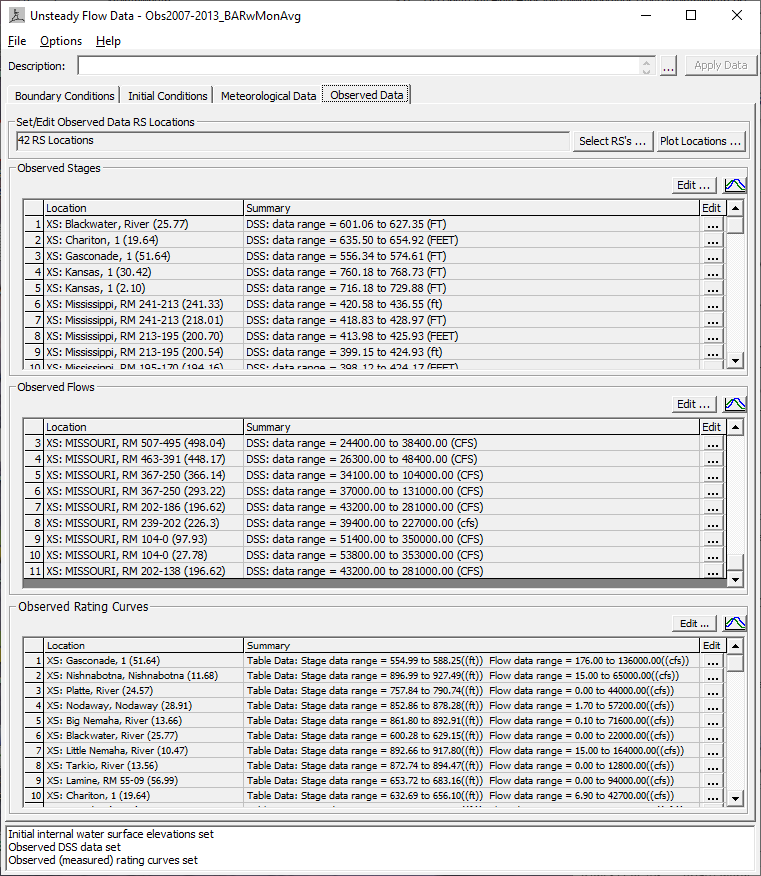
Figure 7 9. Observed Data tab for entering observed data
Once the user has entered locations for the observed data, the next step is to press the "Edit" button above the data type you want to enter (i.e. Observed Stages; Observed Flows; or Observed Rating Curves). If the user presses the Edit button above the Observed Stage or Flow table, a window will appear as shown in Figure 7-10.
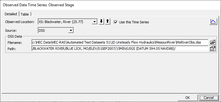
Figure 7 10. Observed Stage Time Series Editor
As shown in Figure 7-10, the window has two tabs. A "Detailed" tab and a "Table" tab. The detailed tab allows the user to view and edit data for one location at a time. The Table Tab allows the user to see the information for all the observed data locations. Whether you view the data in the detailed or table view, the user must first select a Source for the data. The "Source" options are: DSS; Table; Constant. Selecting DSS means the user has the observed data stored in an HEC-DSS file and wants to read the data from that DSS file. Selecting Table means the user wants to enter the data into a table directly in this editor. Selecting Constant means the user only has a "High Water Mark" for this location and wants to enter that High Water Mark as a "Constant" value. High Water Marks will be discussed in more detail below.
There is also an option called "Use this Time Series". This option must be turned on for all observed data that you want to be used for a run. If this option is not turned on, then it will not be used during the run and the user will not be able to plot the observed data against the computed results in any of the plots.
If the DSS source is selected, then the user must select the DSS file to use from the Filename chooser, as shown in Figure 7-10. Then the user must select the specific DSS pathname that contains the observed data. The DSS filename and location, as well as the DSS pathname can be cut and pasted into these fields.
If the Table source is selected, then the window will add a table for entering the data. An example Table is shown in Figure 7-11 below.
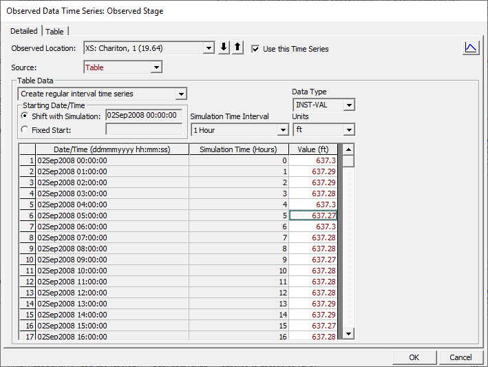
Figure 7 11. Table for entering Observed Time Series Data.
As shown in Figure 7-11, the table has a drop down at the top. This drop down allows the user to select how they want to enter the data. The options are:
Create Regular Interval Time Series: This option allows the user to enter the observed data at a regular interval, such as 1 hour, etc… The user can select to have the Observed data start at the beginning of the simulation time (Which is based on the time window for the run) or they can select to enter a fixed start time for the data.
Enter Date/Time in All Rows: This option allows the user to enter the data as irregular data, meaning the dates and time are not on a regular interval. For this method, the user must enter the data/time for all the observed values.
Enter Simulation Time in All Rows: This option allows the user to enter the simulation time
Additionally, the user must select the Data Type; Time Interval; and the Units of the data. The Data Type can be: INST-VAL; PER-AVE; or PER-CUM. "INST-VAL" stands for instantaneous values, which is the most common for this type of data. "PER-AVE" stands for Period Average data, which means that the data is and average over the time period. "PER-CUM" stands for Period Cumulative, which means the data are cumulative values over the time period, and they are stored with a date and time at the end of the time period. PER-CUM does not make sense for observed time series data, but it is used for other data types, such as precipitation data.
If the Constant value is selected for the "Source" of the data, the window will change and only require the user to enter is single value and the units of that value.
High Water Marks
To enter Observed High Water Marks into HEC-RAS, select the Edit within the Observed Stages area, then select the Constant values as the data source. The editor will like what is shown in Figure 7-12
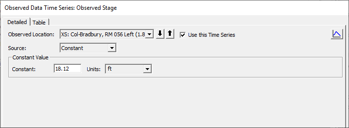
Figure 7 12. Observed High Water Marks entered ad Constant values.
If the high water mark is not exactly at one of the user entered cross section locations, then the user should pick the cross section just upstream of the observed location and then enter the distance from that cross section to the observed high water mark under the column labeled Dn Dist.
Observed Rating Curves
To use the Observed Rating Curve option, the user presses the Edit button within the Observed Rating Curves portion of the window (Near the bottom). When this button is selected a window will appear as shown below in Figure 7-13.
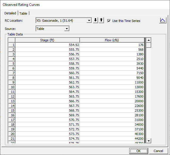
Figure 7 13. Observed Rating Curve Editor.
As shown in Figure 7-13, the user can either enter the data in a Table, or it can be read in from DSS.
Water Temperature (for Unsteady Sediment).
This option allows the user to put in a time series of water temperature data to be used in conjunction with the Unsteady Flow Sediment Transport capabilities. Water Temperatures are used for Fall velocities in computing sediment deposition.