Spatial Results

Similar to 1D and 2D model results, pipe network results are spatially plotted in the RAS Mapper. When a modeling simulation containing a pipe network completes, four new default map layers are added to the map window : Pipe WSE, Pipe Depth, Percent Full, Pipe Velocity. 

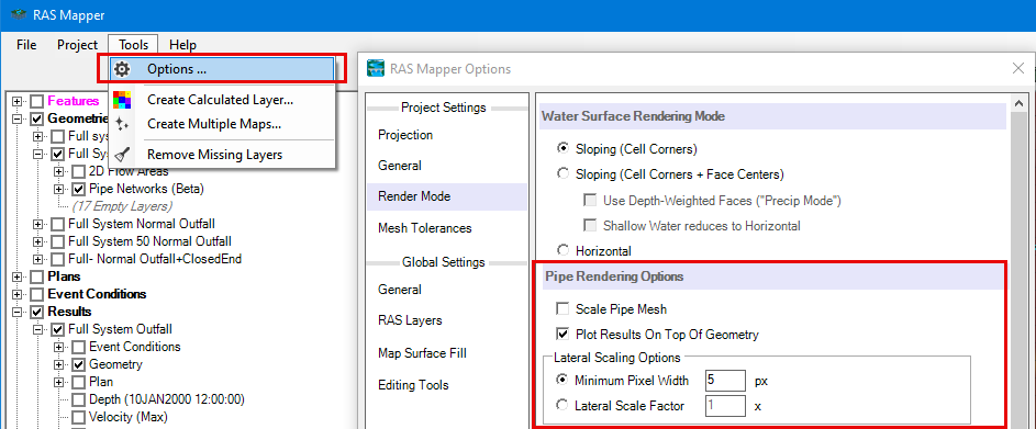
Since the size of stormwater pipes is often very small compared to the surface geometry or model domain, the results be hard to see or become obscured by other model results and geometry elements. To improve the visualization, default render options are provided to laterally scale the pipe results so they can easily seen when zoomed out. Another default option allows pipe results to display on top of surface model results for easier visualization. These options can be accessed through the Tools > Options > Render Mode as shown below.

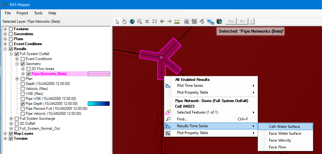
Interpolated pipe results time series can be queried by right-clicking anywhere on the pipe results, and selecting Plot Time Series as shown below. Note that the desired result layer must be checked in the tree view to access the time series. 

In addition to the interpolated spatial results, compute engine results for cells and faces can be accessed by selecting the Pipe Network layer in the tree view, and right-clicking the cell or face in the pipe mesh, as shown below.

Profile Plots

There are a few options for accessing results profile plots for the pipe network simulation, depending on how you want to select which conduits to view in the plot. 

The first option is to launch the profile plot and  subsequently select the individual conduit to plot from the table. This option is good for smaller systems where accessing the desired conduits from the table isn't a burden. This option can still be used for larger datasets, as long as the Major and Minor Groups are setup on conduits, in which case you can access them easier by filtering or sorting the table in the profile plot. A demonstration of accessing the results profile plot this way is shown below.

The other option for accessing the profile plot is to select the desired conduits from RAS Mapper before launching the plot. To do this, select Conduits layer in the tree view, then begin selecting conduits using the select tool. 

Tip

You can add and remove individual conduits from your current selection by holding Ctrl while clicking (both in RAS Mapper and the Profile Plot table).

There are also options to select all Upstream Conduits, select all Downstream Conduits, and select all the conduits that belong to Major and Minor Groups under the Show Conduits option when a the conduit is right-clicked. This option for accessing the result profile plot is shown below. 

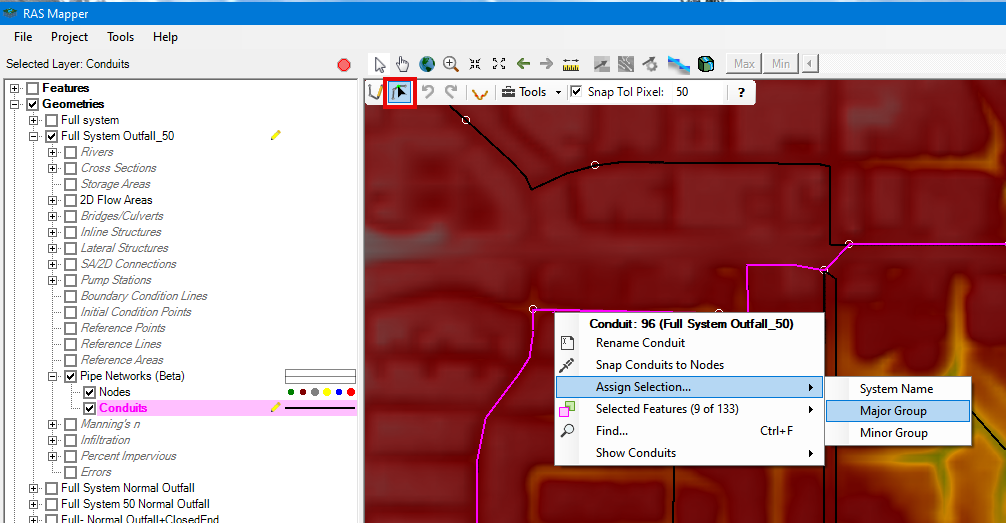
Major and Minor Groups can be set for easier access to conduits by editing them in the attribute table wen in edit mode, or by spatially selecting the conduits and accessing the Assign Selection... menu from a right-click, as shown in the figure below. 

Note

After creating Major and Minor Groups in RAS Mapper, the model will have to be rerun before they can be used for output.

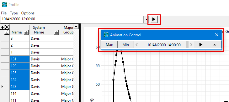
The profile map can be animated via the pop-out animation pane at the top, or can be animated using the controls from RAS Mapper. The benefit of using the controls in RAS Mapper is that all results (profile plots, hydrograph plots, and spatial results will be synched. 

Stage and Flow Hydrographs

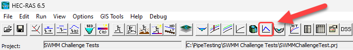
Stage flow hydrographs are available for both Pipe Nodes and Conduits, and they can be accessed from the main HEC-RAS Interface or RAS Mapper. 

When stage and flow hydrograph plot opens, the correct Type will have to be selected from the Type menu as shown below.

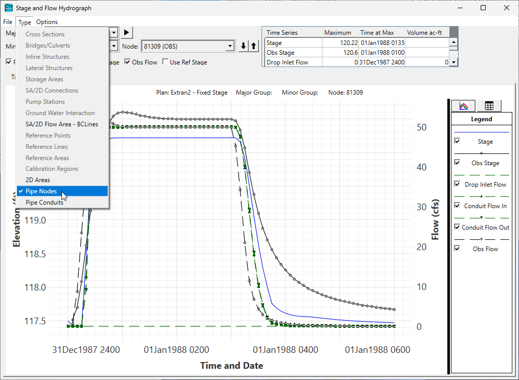
The stage and flow hydrograph plots will  by default inflows and outflow to nodes from conduits, inflows from drop inlets, stages, and observed data (if defined).