Download PDF
Download page Evaluating RAS Results.
Evaluating RAS Results
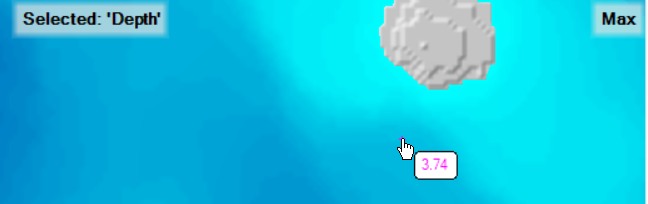
Every effort has been made in HEC-RAS to give the user a consistent interactive experience. However, because of the different data requirements for 1D and 2D modeling, the output options in RAS Mapper will depend on the model type. The simplest method for interacting with HEC-RAS results is to move the mouse cursor over the Map Window and a map tip with the interpolated value value for the Selected Layer with be displayed next the cursor. The selected layer will be highlighted in the Layer List and the name will be shown in the Map Window. The selected Profile will also be displayed ( upper right corner) in the Map Window. The number of decimal places used to show the value is controlled by the Display Output Decimal Places in the Global Settings | General options.
The simple cursor reporting of values is a quick way to get an answer or two, but is reliant on the user selecting the layer of interest and then moving the mouse. More efficient tools are available to analyze the full scope of the HEC-RAS results using the Layer Watch List, Time Series Plots, and Profile Plots.
When querying results Maps, an interpolated value is reported to the user. The interpolated value may change based on the Render Mode and zoom level.
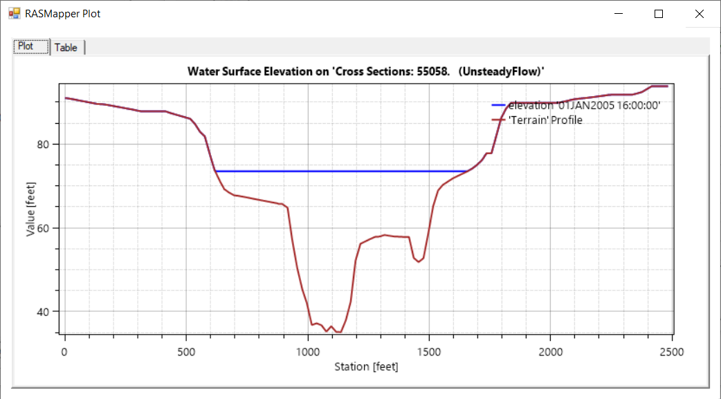
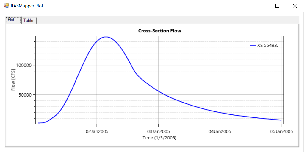
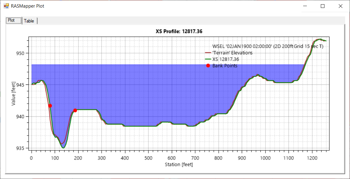
For computed model results (that are not interpolated), you can use the structure of the geometry to query results. For 1D models, this means that the River, Cross Sections, and Storage Areas have results that can be plotted. Select the layer, right-click on the feature and choose the Results Profile Plot option of interest (WSE, Depth, Velocity) or a Results Time Series (Flow, Stage). For 2D models, the 2D Mesh is allows you to select various time series plots for the cell or cell face (discussed in detail, later). Below are an examples for different cross section plot options.
When querying model geometry for Results, such as cross sections or 2D cells, the value computed by the computation engine is reported to the user.
Results Profile Plot for Water Surface Elevation
Results Time Series Flow Plot
Cross Section Terrain Profile Plot
Layer Watch List
The Layer Watch List is provided for the user to simultaneously evaluate multiple layers. This is extremely convenient for diving deep into the results. To use the Layer Watch List, right click on  Add Watch to Layer Values. Each layer will be added to the Layer Values tab, shown below, in the lower left of the RAS Mapper interface. As you add layers, they will automatically be turned on, but you can establish the order you want to the reported values and you can specify the short ID tag next to each value. By default, the first letter of the layer name is used for the ID tag. The Layers Values list also allows you to Add and Delete layers to watch. If you would prefer, you can also
  pop the window out and place it at any desired location.
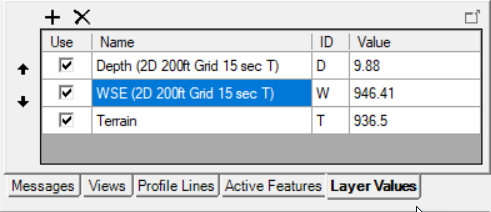
As you move the mouse over the Map Window, values for the watch layers will be shown as the map tip, without having to select the layer. In the example below, the Depth (D), Water Surface Elevation (W), and Terrain (T) are being evaluated. The number of decimal places used to show the value is controlled by the Display Output Decimal Places in the Global Settings | General options.

Time Series Plots
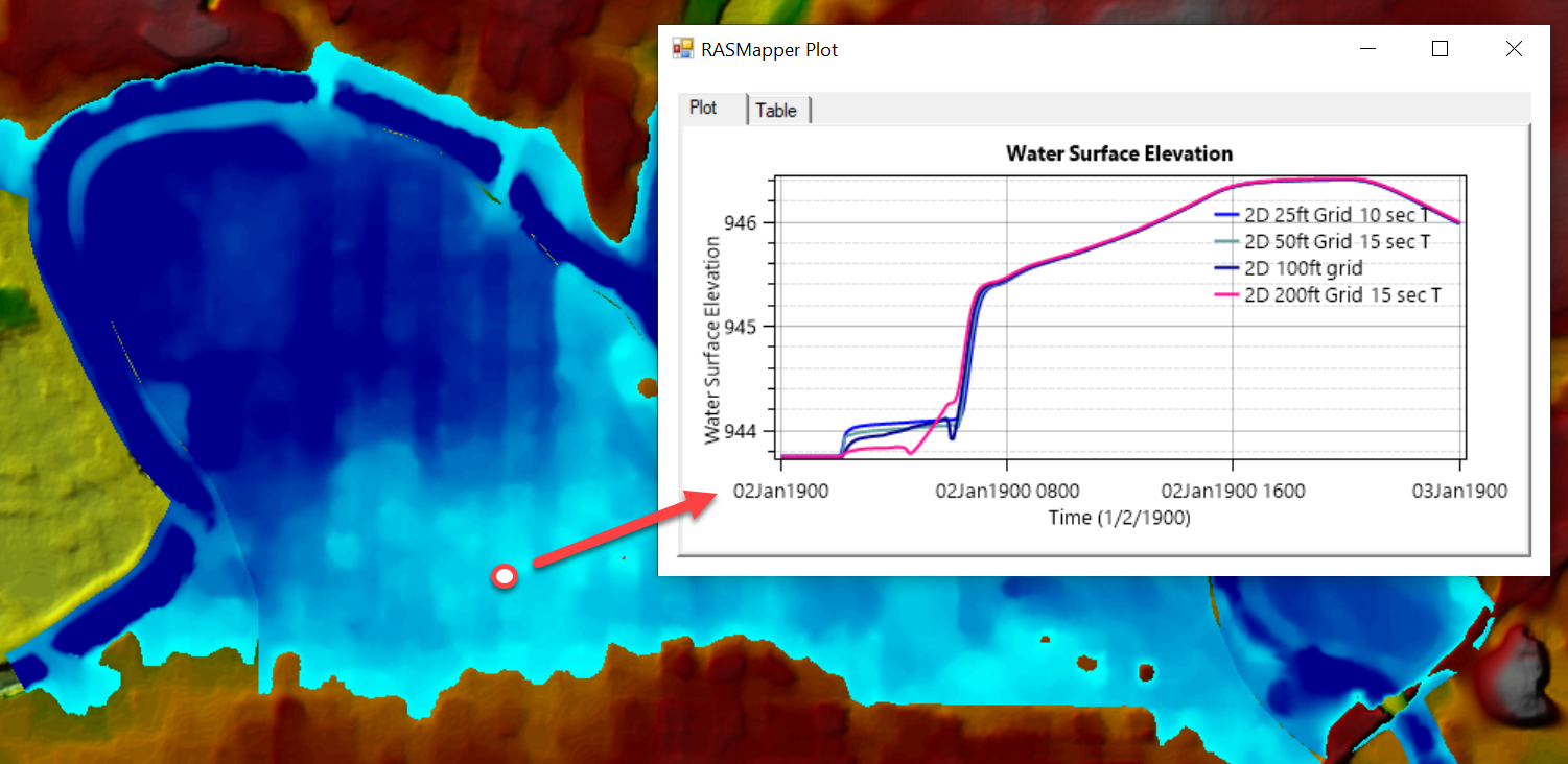
For both 1D and 2D result maps that are enabled there will be a floating menu to plot All Enabled Results | Plot Time Series for WSE, Velocity Depth, and Courant for the current mouse location. The plotted results are based on interpolation of results. If no maps are turned on, the context menu will show the property followed by “[No enabled maps]”. The An example stage hydrograph plot for a location in the model domain for multiple plan results is shown below. The location for which the results are plotted will be highlighted in the Map Window and allows for interactive comparison of results from multiple plans.
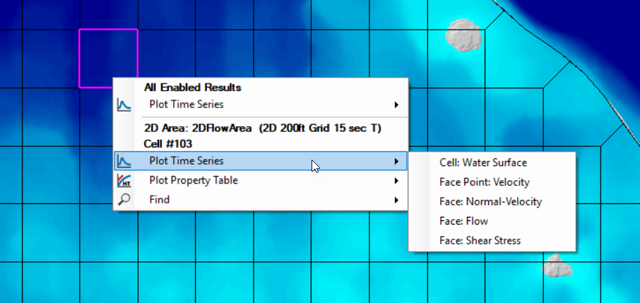
If the 2D Flow Area layer is enabled (turned on, you can see the mesh), as the mouse is moved over the map, the selected cell will be highlighted. A right mouse click provide access to simulation results (not interpolated) for the highlighted cell or cell face. Depending on the zoom level, the mouse will snap to the cell or face (zoom in more to snap to cell center). These computation values are what are used in the 2D hydraulic computations and are available under the Cell/Face Plot Time Series menu option. Available options are listed below.
- Cell: Water Surface
- Fact Point: Velocity
- Face: Normal Velocity
- Face: Flow
- Face: Shear Stress
Not only will a right mouse-click provide access to simulation results, the user will also have access to the pre-processed geometric data. The context menu will provide a Plot Property Table menu item for several plot options.
- Cell: Volume-Elevation
- Face: Profile
- Face: Area-Elevation
- Face: Wetted Perimeter-Elevation
- Face: Manning’s n – Elevation
- Face: Conveyance - Elevation
Profile Lines
River and Cross Sections lines allow you to plot 1D model results, simply by clicking on the feature. However, user-defined Profile Lines allow you to create lines for 2D models in specific locations where you would like to repetitively evaluate simulation results. The Profile Lines layer and is located in the Features group so that the layer is drawn on top of all other features. Profile lines are created using the RAS Mapper Editing tools. To create them, start editing the Profile Lines layer, and create lines wherever you would like to extract information from a raster dataset. The orientation of the profile lines with have zero-station at the start of the line and positive flow will be evaluated with downstream (positive flow) established with the starting point on the left of the line.
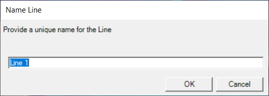
Once a feature has been created, you will be prompted for new name for the Profile Line.
Profile lines are features just like any other in that they can be modified, moved, and deleted. You can also interact with them when the Profile Lines layer is selected. To plot information along a profile line, select the Profile Lines layer and select a feature from the Map. Alternatively, you can select profile line from the Active Features list or the dedicated Profile Lines list. A right-click will allow you to Plot Profile or Plot Time Series.
Plot Profile
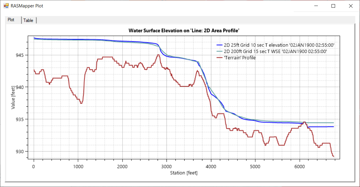
Plot Profile will allow you to create a plot underneath the line for a single mapping time step. Plot options are dictated by what Result layers are turned on in the Layer List (WSE, Depth, Velocity, etc.). There are plot options to plot the map values with and without Terrain. The profile plots are also linked to the animation tools, so you can move through the simulation window to evaluate results. When animating, the profile line and map layer will update. As shown in the figure below, multiple map layers of the same type can be plotted at the same time (so long as they are turned on). The data behind the plots are available for inspection by clicking on the Table tab in the plot.
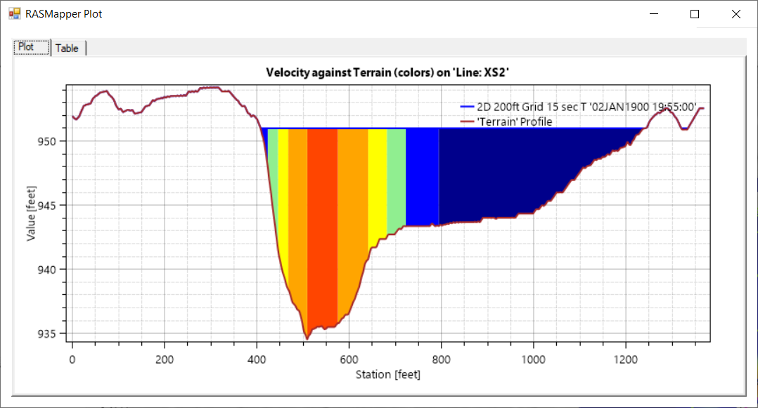
Another plot option when plotting velocities is to plot Velocity with Terrain.
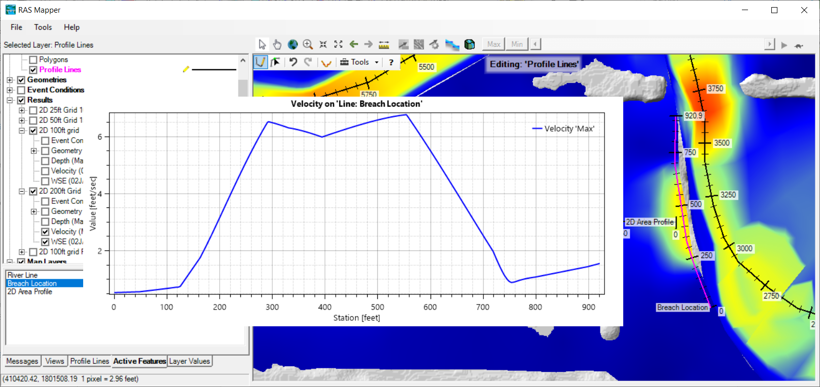
It is also convenient to have an idea where you are along a line. One of the Profile Lines layer plotting properties is the ability to turn on Stationing Tick Marks along the line. In the figure below, a plot of velocities near a breach location are shown along with the stationing along the profile line used to extract the velocity information.
Plot Time Series
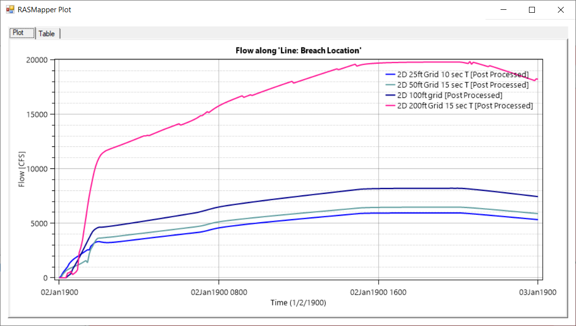
Time series information is also available for a profile line. Option to plot Flow, Volume Accumulation, and a Rating Curve are available. Positive flow is evaluated as flow passing though the line (away from the viewer) when looking at the line with zero-station on the left. An example plot comparing flow through a breach location is shown below.
Creating Vector Contours
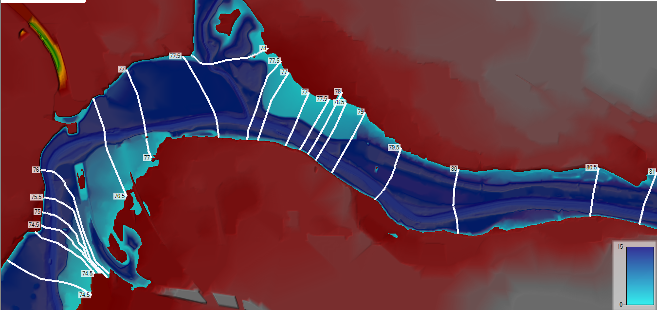
Contours can be created for all RAS Results and saved to a shapefile. To create contours, right-click on the result (e.g. WSE Layer) and select the Export Layer | Create Vector Contours menu item. In the dialog provided, choose the computational extent, contour interval, and filter tolerance (to help reduce the number of point for each contour line for big datasets).
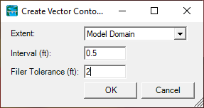
Click OK and provide a filename in the dialog provided.
Contours will be generated and added to RAS Mapper. You can then configure the labels and edit, as desired. An example set of contours for WSE draped over the depth grid and terrain is shown below.