Managing Results Maps

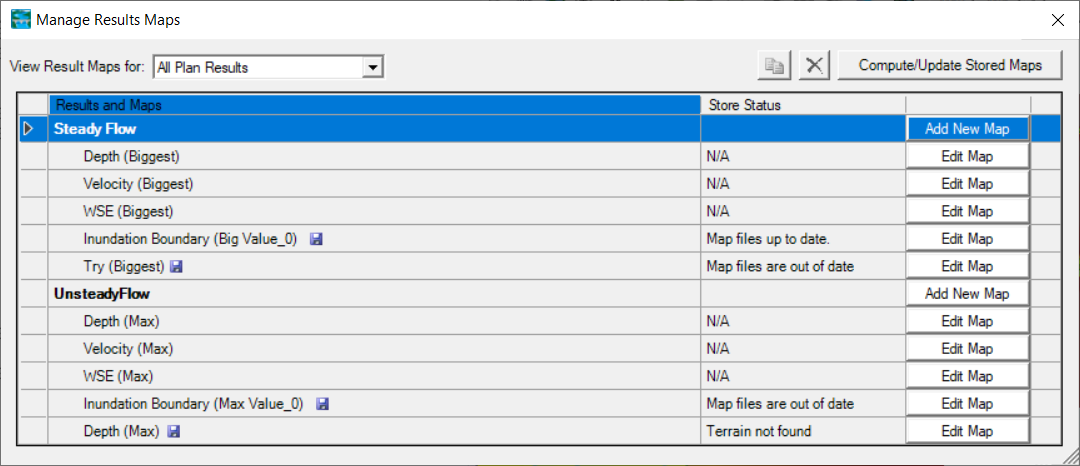
Once a Results Map has been created, it is listed by Plan in the management dialog. The Manage Results Map dialog is available by right-click on the Results group. It organizes data by Plan and identifies which maps are dynamic or stored, and provides a message on the status of the map.  If the layer is a stored map, but has not yet been processed, the label “Map not created yet” will be shown under the “Store Status”.  To compute a stored map, select the layer in the list (multiple layers can be selected by holding the Ctrl key) and press the Compute/Update Stored Maps button on the Manage Results Map Dialog. As the map results are computed, a status message will be provided updating the user with the progress.   Upon completion, the status label will change to “Map files up to date”.  There are also options on the dialog to Copy and Delete a results map.

The Manage Results Maps dialog is convenient for processing multiple stored maps.

RAS Results

As long as a Terrain Layer is associated with a Plan, dynamic results layers for Depth, Velocity and Water Surface Elevations will be available. Results for each plan are stored in an HDF file.  This HDF file has a copy of the input geometry and computed values from the HEC-RAS simulation.  When RAS Mapper loads, there will be a node in the Layer List for each Plan.  For each Plan, layers are created for the input Geometry, Depth, Velocity, and Water Surface Elevation (WSE).

Each result maps can be evaluated by selecting the layer and hovering the mouse over a selected location.  The selected map will be shown in Magenta in the layer list.  If the map is a dynamic map, it can be animated using the animation toolbar.  The animation tool will allow the user to plot the Maximum or Minimum profile, step through each profile, or play the entire set of profiles.  The water surface Profile (time step) selected by the animation tool will be displayed in the corner of the Map window.

Animation of multiple layers is accomplished by selecting a Plan of interest.  All layers that are currently displayed (checkbox is turned on) will have the profile updated to match the time step of the animation tool.  Layers that are not turned on will not have the profile updated.  Animation of multiple layers from different Plans (for Plan comparison) is accomplished by selecting the “Results” node in the Layers List.  The first Plan (“base” Plan) turned on will be used to establish the time step of the Animation Tool.  Any Profile of displayed layers (from Plans that are turned on) that matches the base Plan Profile will be updated. 

Interpolation Surface

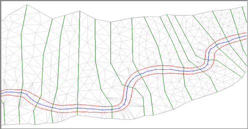
Geospatial analysis and visualization of the HEC-RAS results will be based on the Interpolation Surface.  The surface is created differently for 1D and 2D model domains.  For a 1D model, the Interpolation Surface is created based on River, Bank Lines, River Edge Lines, and Cross Section layers. The shapes of the River lines and Bank Lines are used create the Edge Lines (which connect the ends of the cross sections).  These three line features will act as transition lines to interpolate hydraulic results from cross section to cross section.

Four interpolation “regions” are then created based on triangulation between each set of cross sections using the transition line features (River, Bank Lines, River Edge Lines): (1) between the left river edge line and the left bank line; (2) between the left bank line and river centerline; (3) between the river line and right bank line; and (4) between the right bank line and the right river edge line. The interpolation surface created between each set of cross sections becomes the XS Interpolation Surface that RAS Mapper uses to determine how to distribute computation results from cross section to cross section for each region.  An example interpolation surface is shown below.

The limits of the Interpolation Surface is dependent on the Edge Lines that connect the ends of the cross sections.  You can only edit the Edge Lines in the Geometry (not the Geometry in the Results!), because editing should be performed prior to model simulation.  After simulating, if you want to change the Edge Lines, you can import them from an existing Geometry.  This is accomplished by right-clicking on the Geometry node and selecting the Import Edge Lines and Recompute Interpolation Surface menu item. The newly imported Edge Lines will be display along with lines that show what HEC-RAS computed to be the limits of the model based on the cross sections.  User-modified Edge Lines is not intended to fix model limitations, rather to improve small areas where base mapping functionality was deemed deficient.  Water surface elevations, velocities and other hydraulic results will not be the same as results from a refined model with improved cross sections.

For 2D models, interpolation is performed based on triangulation between computation points and face points.  How the interpolation is performed; however, is slightly different based on the Render Mode when evaluating Map Type (water surface elevations versus velocities). Further, there are three Render Modes available within RAS Mapper: (1) Hybrid, (2) Sloping, and (3) Horizontal.  These Render Modes are available from the Options | Render Mode menu item or by clicking the Render Mode button.  The Hybrid method is the default method and is a combination of the Sloping and Horizontal methods. The render mode will affect both the dynamic map and the store map results.

• Hybrid - This method attempts to employ the most appropriate rendering method based on the flow conditions. This is the default rendering mode.
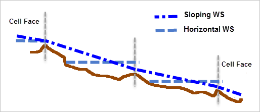
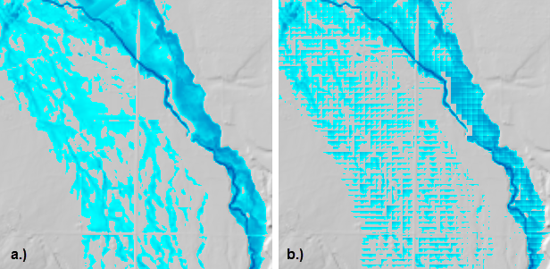
• Sloping Water Surface  – The Sloping water surface rendering mode plots the computed water surface by interpolating water surface elevations from each 2D cell face.  This option of connecting each cell face provides a visualization for a more continuous inundation map.  The more continuous inundation map, looks more realistic; however, under some circumstances it can also have the appearance of more water volume in the 2D cells than what was computed in the simulation.  This problem generally occurs in very steep terrain with large 2D grid cells.  This sloping water surface approach is most helpful when displaying shallow inundation depths in areas of steep terrain. This method is not a volume conservative approach.  Water most likely will "be created" during the interpolation.
• Horizontal Water Surface – The Horizontal water surface rendering mode plots the computed water surface as horizontal in each 2D Area cell.  This option fills each 2D cell to the water surface as computed in the 2D simulation.  In areas where the terrain has significant relief between 2D cells this plotting option can produce a “patchwork” of isolated inundated areas when visualizing flood depths.  These isolated inundation areas are more visible in areas of steep terrain, using large grids cells, with shallow flood depths.  This method is a volume conservative approach and should be used to generate stored maps where water volume will be used for further calculations.

A comparison of the Sloping and Horizontal water surface methods is shown below.

The impacts of the two different render modes are shown based on inundation depth in the figure below.

Water Surface Elevation

A surface of water surface elevations is created using the the interpolation surface.  If present, Storage Areas and 2D Flow Areas will take precedence over Cross Sections.  For 1D models, water surface elevations are inserted into the surface at cross sections.  For 2D models, water surface elevations are inserted at the location of computation points.  An example water surface elevation map is shown below.

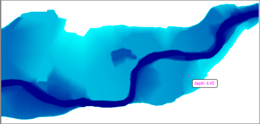
Depth

Water surface depth is computed based on the difference in water surface elevations and the terrain elevations.  The values reported to the screen for dynamic maps will be based on the resolution of the map you are looking at.  If you are zoomed out, you will be not be looking at the "exact" value based on the simulation, rather a values based on the resampling of the terrain and water surface based on the pyramid level you are zoomed to.

Inundation Boundary

The Inundation Boundary map type generates a polygon boundary at the zero-depth contour when comparing the water surface elevation to the associated Terrain layer.  This layer is a stored dataset that is developed for a specific water surface profile.  An example flood inundation boundary map is shown in below.

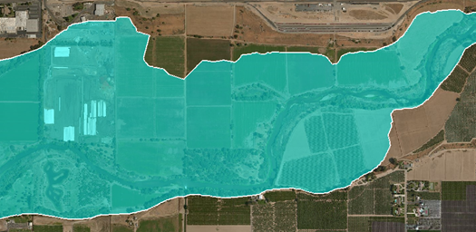
The inundation boundary for various depths can be evaluated by selecting the Map Type of Depth, Max Profile, and setting the Polygon Boundary Value to the depth of interest. 

Note: This is approach allows for the evaluation of depths less than or greater than zero for 1D models; however, it is only able to evaluate depths greater than zero in the 2D domain.

Editing the Inundation Boundary

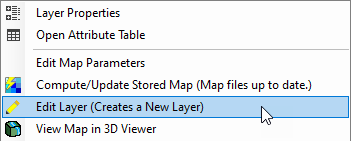
The flood inundation boundary that results from the HEC-RAS simulation and mapping may not result in a hydraulically correct flood map.  Errors may result from limitations in terrain or model geometry.  You can improve the final flood map using the standard editing tools provided in RAS Mapper.  To start editing, right-click on the inundation boundary layer and choose the Edit Layer menu item.  The original inundation boundary layer is a multipart shapefile and will not work with the singlepart vector editing tools in RAS Mapper.  Therefore, as shown in the image of the menu item, this process will Create a New Layer.

The new layer will be created and added to the map below the original inundation boundary layer, as shown below.

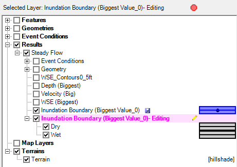
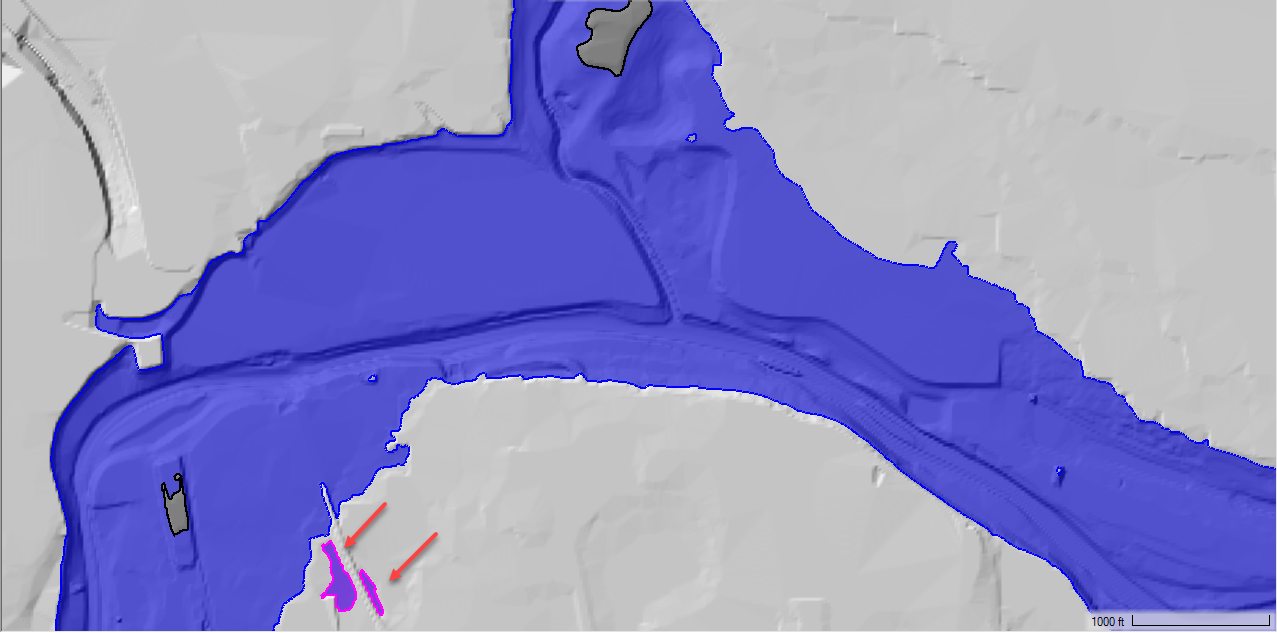
The new layer (designated with the "-Editing" suffix) will be comprised of two child layers that comprise the "parts" and the "holes" of the multipart inundation boundary.  The "parts" are labeled as "Wet" and the "holes" are labeled as "Dry".  At this point, select either the Dry or Wet layer to edit those features individually.

Select the Dry layer to remove small holes in the floodplain.

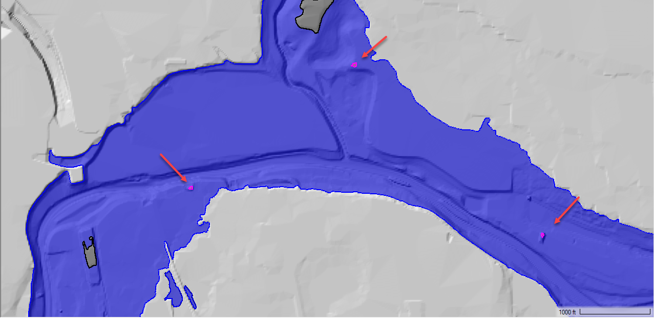
Select the Wet layer to improve the floodplain boundary or to remove areas that should not be inundated.

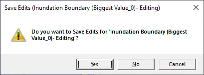
When finish editing, Stop Editing and choose to save the edits.

The final inundation boundary layer  (designated with the "-Modified" suffix) will again be a multipart shapefile created from the individual wet and dry layers.

Editing the Edge Lines

Often, you will wan to make edits to the floodplain and have them persist through each simulation.  Review model which has a levee system will result in inundation mapping inconsistencies.  No amount of cross section improvement can adequately satisfy the inundation mapping.  Therefore, RAS Mapper provides the ability to edit the Edge Lines layer. 

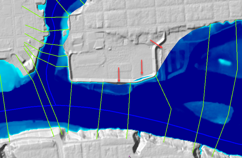
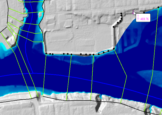
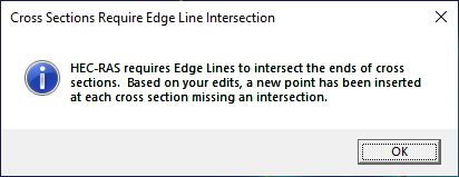
To improve the inundation mapping, edit the Edge Lines layer (grouped under the Cross Sections Layer).  Shown in the figure below, is the Edge Line being edited (grey line with black vertices) to follow a complex levee alignment.  When done editing an edge line feature, RAS Mapper will make sure that the edge lines are connected with the end of the cross sections and provide a warning message that the edge lines are going to be modified (a new point on the end of the cross section will be inserted). 

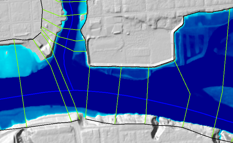
Further, the Edge Lines layer will now be saved in the results output during the simulation. The resulting floodplain mapping is now hydraulically correct, as shown below.

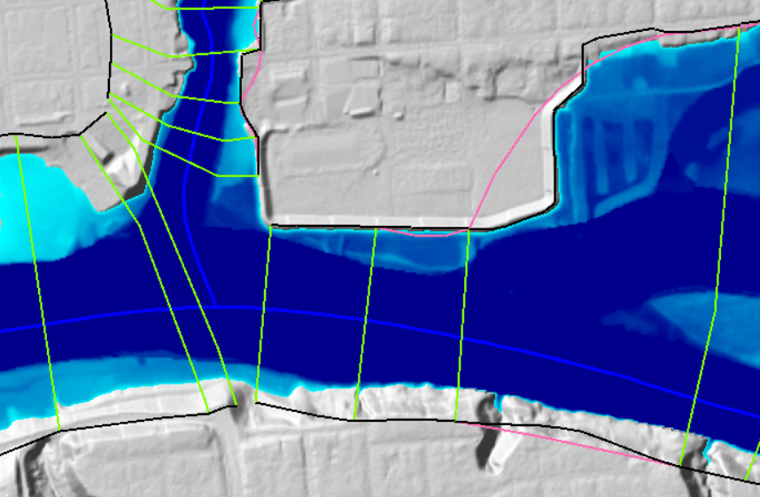
It is often necessary during model review to identify if a modeler has modified the Edge Lines to improve the inundation mapping.  The option to visualize the default model domain boundary is available from the Edge Line Layer Properties by turning on the Plot Default Edge Lines option.

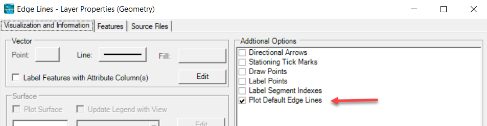
As shown in the figure below of the floodplain, the HEC-RAS computed (default) boundary will be shown in magenta, while the modified Edge Lines are shown in black.

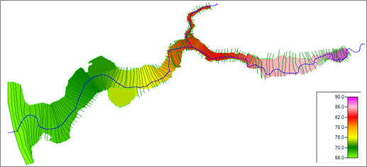
Velocity

1D interpolated velocity results are created using the computed velocities at each cross section.  The number of velocities that are used for interpolation are based on the Cross Section Subsection Distribution specified from the Horizontal (Velocity mapping) option on the HTAB Editor in the HEC-RAS geometry editor. Because the interpolation surface was created based on regions, there will not be any velocity interpolation across bank lines; therefore, overbank velocity data are not interpolated with channel velocity data.  This methodology prevents areas with extreme velocities from influencing the distribution values (low velocity values in the overbank being affected by high velocity values in the channel).  

If velocities are an important model evaluation criteria, a 2D model should be created.  Velocities from 2D model results use the normal velocities at the cell face to create an interpolated velocity surface.  An example velocity magnitude plot is shown below.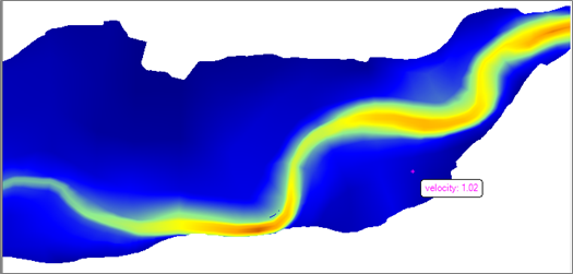 

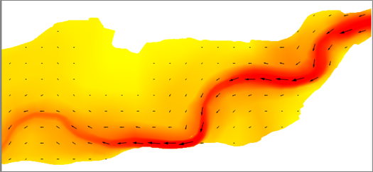
There are several ways to visualize velocity data within RAS Mapper.  Velocity vectors are available by turning on the Plot Static Arrows option.  This will use the magnitude of velocities for determining arrow length and evaluate the interpolation surface for determining the flow direction (again, this is based on the shape of the river and the interpolated bank lines and edge lines).  An example velocity vector surface with static arrows is shown below.

Velocity arrows are plotted on a regular interval based on a user-defined spacing based on screen pixels.  This spacing refers to how often an arrow is displayed (when zoomed in the number should be higher and when zoomed out the number should be lower). The user can also specify to the color the arrows in black or white.  This parameter is available by clicking on the   Edit Velocity Parameters option.   

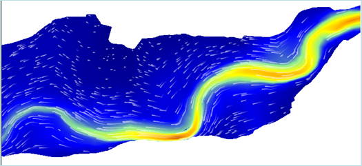
HEC-RAS also has the capability to visualize the movement of flow using Particle Tracing.  To see an animation depicting the relative flow velocity and direction, click on the   Particle Tracing option.  The flow lines are generated by using the velocities on the depth grid to move a particle along the interpolation surface during animation.  A trace of the particle will be created based on the distance and direction it has moved during the animation and will give the appearance of stream lines.  An example plot of the Particle Tracing capability is shown below.

Depending on the zoom level, complexity of the floodplain, variation in velocities, and personal preference the user may need to adjust velocity trace parameters. Options for the particle trace are available by right the  Edit Parameters option.  Particle Tracing options include Speed, Density, Width, Lifetime, and Anti-Aliasing.  A description of velocity mapping options is summarized in the table below.

Once a Results Map has been created, it is listed by Plan in the management dialog. The Manage Results Map dialog is available by right-click on the Results group. It organizes data by Plan and identifies which maps are dynamic or stored, and provides a message on the status of the map.  If the layer is a stored map, but has not yet been processed, the label “Map not created yet” will be shown under the “Store Status”.  To compute a stored map, select the layer in the list (multiple layers can be selected by holding the Ctrl key) and press the Compute/Update Stored Maps button on the Manage Results Map Dialog. As the map results are computed, a status message will be provided updating the user with the progress.   Upon completion, the status label will change to “Map files up to date”.  There are also options on the dialog to Copy and Delete a results map.

The Manage Results Maps dialog is convenient for processing multiple stored maps.