Download PDF
Download page Creating Results Maps.
Creating Results Maps
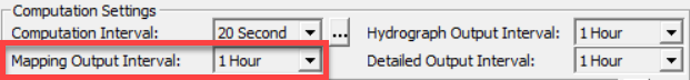
HEC-RAS results are stored in a single .hdf output file based on the simulation Plan information (for example rasproject.p01.hdf). Therefore, an entire copy of the geometry used for the simulation and simulation results are written to the output file. For unsteady-flow simulations, time-series data is written out based on the Mapping Output Interval specified on the Unsteady Flow Analysis window. This Mapping Output Interval is what is used for animating water surface results in RAS Mapper.
When RAS Mapper is opened, the Layer List will automatically add in a result layer for each plan. Layers will be created to allow you to visualize the geometry used to construct the model, various output types, and other data such as event conditions. By default, inundation maps for Depth, Water Surface Elevation and Velocity will be created to assist in visualizing the results. The Result will also automatically be associated with the Terrain layer used to create the geometry - this is necessary to properly compute flood depth and inundation boundary information.
Result Maps
Results are managed in HEC-RAS in two distinct methods: (1) dynamic maps and (2) stored maps. Dynamic maps are generated on-the-fly for the current view and are intended to be the main method for visualizing and interacting with results in RAS Mapper. Each time you pan or zoom the result map is updated based on the view extents and based on the zoom level. This results in a resampling of interpolated data and is NOT the exact (computed) answer for any specific point. Stored maps are written to disk based on resolution of the RAS Terrain and are intended as a permanent data storage solution. Dynamic mapping should be used by the HEC-RAS modeler for hydraulic analysis, investigation, and model refinement. Stored maps should be used to publish and transfer results for use in further analysis outside of the HEC-RAS software. Dynamic mapping and stored maps results will not be exactly the same because the dynamic maps are generated for screen pixels and the stored maps are generated based on the underlying RAS Terrain cell size.
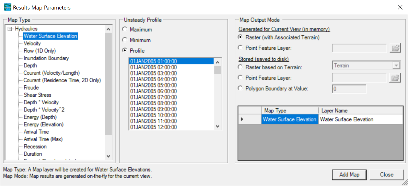
By default, a RAS Result is added to RAS Mapper and dynamic maps for Depth, Water Surface Elevations, and Velocity are automatically generated. Additional maps can be created by right-clicking on a result and choosing the  Add New Results Map Layer menu option. Select the Map Type, Profile, and Output Mode in the Results Map Parameter dialog shown below. Layer Names can also be provided. The Map Type refers to the hydraulic (or sediment) variable to plot, the Profile is the computation time step to evaluate, and the Output Mode is either dynamic or stored. Once the map type and parameters are selected, click the Add Map button to add the map to RAS Mapper. As shown in the figures below, the map parameters will change base on the Map Type selected.
Associated Terrain
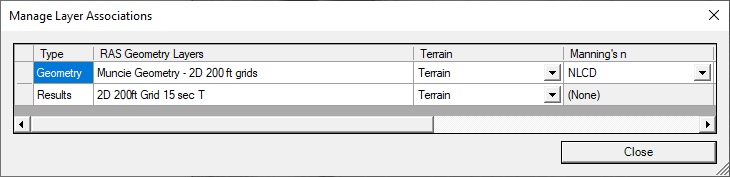
A Terrain Layer must be associated with the RAS Geometry Layer and Results Plan prior to creating a results map. (The Plan must also have been simulated, creating an output HDF file.) If there is only one Terrain Layer in the RAS Mapper, it will be associated with all geometries and results; however, to associate a Terrain Layer manually, right-click on the Results node and select the Manage Terrain Associations menu item. In the associations dialog shown below, select the Terrain Layer for each RAS Result.
The terrain layer is used in the inundation mapping process to compare the computed water surface to the ground surface. Depending on the expanse and resolution of the terrain data, users may have chosen to tile the original terrain datasets to reduce file size and improve computational efficiency using raster (gridded) datasets. The Terrain Layer may be organized as desired by the user; multiple terrain models may overlap, there may be gaps, or a single terrain model may be used for a specific location in the model.
Map Type
The Map Type identifies the type of map that will be created. The available Map types will vary based on the type of simulation performed. For example, an Arrival Time map is not available for a steady-flow simulation. A summary of map types is provided in the table below.
| Map Type | Description |
|---|---|
Depth | Water depths computed from the difference in water surface elevation for the selected profile and terrain. A Terrain Layer must be associated with the Plan. |
Water Surface Elevation | Water surface elevations for the selected water surface profile at all computed locations and spatially interpolated between those locations. |
Velocity | Spatially interpolated velocity results at computed locations for the selected water surface profile. |
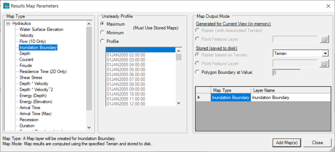
Inundation Boundary | Inundation boundary computed from the zero-depth contour of flood depths for the selected water surface profile. A Terrain Layer must be associated with the Plan. |
Flow (1D Only) | Interpolated flow values as used in the RAS simulation for the selected water surface profile. This option is only available for 1D simulations. |
Courant (Velocity/Distance) | The Courant number is computed as the flood wave velocity times computation time step divided by the distance the wave traveled. For a 1D model, velocity slices are used and distance is computed along the main channel from cross section to cross section. For a 2D model, face velocities are used and distance is computed from computation point to computation point. |
Courant (Residence Time) | The Courant number is computed using a Residence Time - a cell volume divided by net flow out of the cell. |
Froude | The Froude number is computed as the local velocity divided by the square root of the gravitation constant and distance. For a 1D model, velocity slices are used and distance is computed along the main channel from cross section to cross section. For a 2D model, face velocities are used and distance is computed from computation point to computation point. |
Shear Stress | Shear stress computed as: (γRSf). For 1D cross sections, the cross section is broken into user defined slices, then average values are computed for each slice. Values are interpolated between cross sections using the cross section interpolation surface. For 2D cells it is the average shear stress across each face, then interpolated between faces. |
Stream Power | Stream Power is computed as average velocity time’s average shear stress. For 1D cross sections, the cross section is broken into user defined slices, then average values are computed for each slice. Values are interpolated between cross sections using the cross section interpolation surface. For 2D cells it is the average velocity times average shear stress across each face, then interpolated between faces. |
Depth * Velocity | Computed as the hydraulic depth (average depth) multiplied by the average velocity at all computed locations and spatially interpolated between those locations. For 1D cross sections, the cross section is broken into user defined slices, then average values are computed for each slice. For unsteady-flow runs, the Maximum value is the maximum of depth times velocity squared based on the user mapping interval, and not the computation interval. For 2D cells the hydraulic depth is computed for each Face, then multiplied by the average velocity squared across that face. Because the Max computation must evaluate the results for the entire simulation this can be computationally expensive and may take several minutes to generate; therefore, this option is most appropriate for a stored dataset (caution using a dynamic map). |
Depth * Velocity2 | Computed as the hydraulic depth (average depth) multiplied by the average velocity squared at all computed locations and spatially interpolated between those locations. For 1D cross sections, the cross section is broken into user defined slices, then average values are computed for each slice. For unsteady-flow runs, the Maximum value is the maximum of depth times velocity squared based on the user mapping interval, and not the computation interval. For 2D cells the hydraulic depth is computed for each Face, then multiplied by the average velocity squared across that face. Because the Max computation must evaluate the results for the entire simulation this can be computationally expensive and may take several minutes to generate; therefore, this option is most appropriate for a stored dataset (caution using a dynamic map). |
Energy (Depth) | Depth to the energy grade line computed as the combination of water depth plus kinetic energy. |
Energy (Elevation) | Elevation of the energy grade line computed from the combination of water surface elevation plus kinetic energy. |
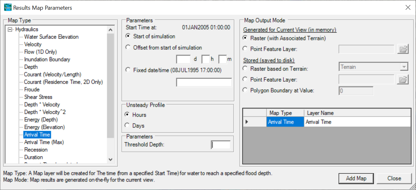
Arrival Time | Computed time (in hours or days) from a specified time in the simulation when the water depth reaches a specified threshold flood depth. The user may specify the time units, start time, and depth threshold. |
Arrival Time (Max) | Computed time (in hours or days) from a specified time in the simulation when the water depth reaches its Maximum flood depth. The user may specify the time units, start time, and depth threshold. |
Duration | Computed duration (in hours or days) for which water depth exceeds a specified flood depth (threshold), The user may specify the time units, a start time, and depth threshold. (Note: RAS ignores multiple peaked events. Once a depth threshold is reached the duration continues until the depth has completely receded for the event.) |
Recession | Computed time (in hours or days) from a specified time in the simulation when the water depth recedes back below a specified inundation depth (threshold). The user may specify the time units, start time, and depth threshold. |
Percent Time Inundated | The amount of time an area is inundated as a percentage of the total simulation time range. |
Wet Cells | Identifies which cells are wet or dry. Partially wet cells are considered entirely wet. |
Profiles
The profile selects the computation time step from which to use data. Profile options will change based on the simulation type (steady/unsteady/sediment) and map type. For instance, for an Arrival Time map, a Threshold Depth and Start Time must be specified.
For steady-flow simulations, the profile group will have a list of all the profiles in the steady-flow file. For unsteady-flow simulations, the Profile group will have the option to choose between Minimum, Maximum, or a specific time step (as set by the ‘Mapping Output Interval’ on the Unsteady Flow Analysis dialog).
Output Mode
The Map Output Mode determines whether the map is Dynamic or Stored. Dynamic maps are recomputed in RAS each time the map extents change based on the zoom level. Further, dynamic maps can be animated within RAS Mapper (assuming there is time series information). Stored maps, however, are computed using the base resolution of the underlying Terrain Layer and stored to disk for permanent access.
RAS provides the option of calculating output values as a raster surface (using the Terrain Layer as the template) or at point locations using a point shapefile as the output template. Often outputting data at specific locations is the prudent course of action to decrease computation times and data storage!
| Map Output Mode | Description |
|---|---|
Dynamic | Map is generated for current view dynamically. Results in the output HDF file may be animated if there are multiple profiles for the variable. |
Raster | Gridded output is computed based on the associated Terrain. |
Point Feature Layer | Values are computed a locations specified by a point shapefile. For the Depth map type, elevation values are compared against the Associated Terrain, Z-Values from shapefile points, or using a specified column for elevation data (in a point shapefile). |
Stored | Computed map is stored to disk. |
Raster | Gridded output is computed based on the user-specified Terrain and stored to disk. The Associated Terrain is the default. |
Point Feature Layer | Values are computed a locations specified by a point shapefile. For the Depth map type, elevation values are compared against the Associated Terrain, Z-Values from shapefile points, or using a specified column for elevation data (in a point shapefile). |
Polygon Boundary at Value | A polygon boundary is created at the specified contour value stored to disk. This is the default option for the Inundation Boundary map type using the computed depth at the zero-depth contour. |
Dynamic versus Stored Maps
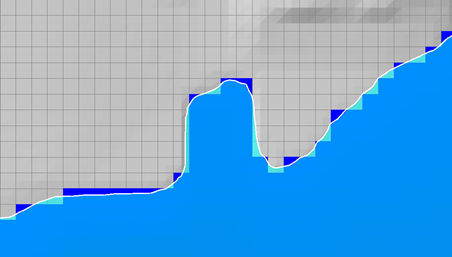
There can be important differences in the computed values between the dynamic results and the stored raster information. Dynamic maps differ in that they are a surface created through the interpolation of values; therefore, as the user moves the mouse in the display the interpolated value for the corresponding location will be displayed. This is in contrast to viewing a raster in a typical GIS where the reported value (from a stored map) will be that for the entire grid cell.
For dynamic depth results, the values reported to the user at a specific map location may change depending on the zoom level. This is because for dynamic mapping, the terrain pyramid level used for evaluating the ground surface elevation is dependent on how far the user has zoomed in or out on the map. Even while zoomed in so that the base data are used for analysis, the map results will not be identical, especially at the floodplain boundary. This is because for the stored depth grid the cell is considered either wet or dry. For a dynamic map, the flood boundary is determined by interpolating the elevations values and intersecting the interpolated water surface with the interpolated terrain elevations for the boundary. The dynamic map will, therefore, result in a “smooth” floodplain boundary. An example of the differences between the dynamic mapping and stored mapping are shown below.
Creating Multiple Maps
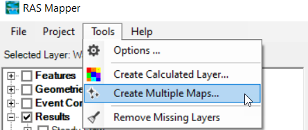
After diligently modeling various flow scenarios, evaluating dynamic map results, and refining the model, you may want to create multiple maps stored on disk. Rather than create the maps individually, you can create a library of multiple stored maps using the Tools | Create Multiple Maps option.
The Create Multiple Maps option allows you to select multiple Plans, Profiles, and Map Types for datasets you wish to store to disk. Further, the window provides an options to Add Maps to RAS Mapper (it is turned off by default as most likely you just want to publish the stored maps). You can use the Ctrl and Shift keys to make multiple selections. Note that for unsteady simulations, you need to have comparable time steps, if you wish to do multiple profiles.
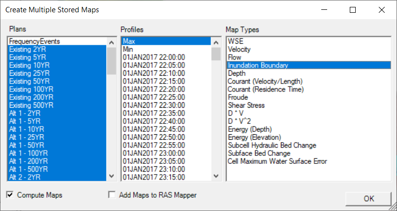
After you have made the Plan, Profile, and Map Type selection, press OK to generate the stored maps.