Download PDF
Download page Workshop 2 – Basic Guide Curve Operations .
Workshop 2 – Basic Guide Curve Operations
Last Modified: 2023-02-09 13:58:44.517
Software Version
HEC-ResSim pre-release Version 3.5 will be used during the 2023 PROSPECT #098 course. Download here: https://drive.hecdev.net/share/YETr0az6
Workshop Instructions (PDF): Workshop 2 - Basic_Guide_Curve.pdf
Download Initial Zipped Watershed: WS2_Start.7z
Download Zipped Workshop Datafiles: WS2_data.7z & CrazyMountainData.xlsx
Download Solution Zipped Workshop: Workshop 2 - Basic_Guide_Curve_Solution.pdf & WS2_Solution.7z
Introduction
The objective of this workshop is to demonstrate how to construct and use alternatives. Alternative construction is fundamental to the development of a simulation and its subsequent analysis. You will also analyze the results of the simulation to gain an understanding of the basic guide curve operation.
Problem Description
You will start this workshop with the “solution” watershed from Workshop 1. In that workshop, you developed a reservoir network for the Ventura River basin and the Crazy Mountain reservoir.
In this workshop you will:
- Create a Basic Guide Curve Operation set at Crazy Mountain Reservoir
- Create an alternative that will use the existing network and operation set
- Define the lookback (initial) conditions and attach time series data
- Create a simulation in the simulation module
- Compute varying alternatives and analyze results
This workshop will use functions from the Reservoir Network Module and the Simulation Module. The references (CrazyMountainData.xls and CrazyMountainRegManual.pdf) from Workshop 1 will be used in this workshop also.
Tasks
1. Copy dss file
from C:\class\Workshop 2 – DSS Data to C:\class\My Watersheds\WS2_Start\shared directory using Windows Explorer.
2. Start ResSim
and open your starting watershed: WS2_Start.
3. Create a Basic Guide Curve Operation Set
- From the Reservoir Network module, select the Network menu and Open the 01 Standard
- Open the Reservoir Editor by selecting Reservoirs… from the Edit
- Select the Operations tab and select Operations_New from the menu bar. Name the new operation set as Basic GC, add a description “Basic Guide Curve Operation”, and press OK. (A set of default reservoir zones will be generated and a zone tree will appear.)
- Right-click on the Flood Control zone in the zone tree and select Rename… Rename the zone to “Normal Flood Control”.
- Add three more Zones: Top of Dam, Major Flood Control and Drought Contingency by selecting New… from the Zone Menu at the top of the Editor.
- Click on each zone and fill the corresponding Date-Elevation information provided in the xls spreadsheet under the “WS#2 Basic Guide Curve Oper Set” tab. If the top elevation does not change throughout the year, then enter the value for 01Jan. (Section III of the Regulation Manual also shows the reservoir zone definitions for Crazy Mountain Lake.)
- Press OK to apply changes and close the reservoir editor.
Tip
By default, the top of the Conservation Zone is used as the Guide Curve. The Reservoir Editor (Operations tab, Zone-Rules sub-tab) gives a visual clue to the zone used for the Guide Curve by displaying its name in bold type. You can assign the Guide Curve to the top of another zone by right-clicking on the desired zone and selecting Set Guide Curve from the popup menu.
- Save the Network and the Watershed by selecting Network > Save and then File > Save Watershed from the menu bar.
4. Create an Alternative
- In the Reservoir Network module, click on Alternative in the menu bar and Edit… to open the Alternative Editor. Create a NEW alternative (click on Alternative in the menu bar and New…) based on the “01 Standard” network, and name the alternative “GC_ops” and give a description.
- In the Alternative Editor, notice that the “01 Standard” network has been associated with this alternative. Under the Run Control tab, choose the desired time step (1Hour) and flow computation method (Instantaneous).
- Select the Operations tab in the middle of the window. For the reservoir, select the Basic GC operations set. Save the alternative.
- Select the Lookback tab. Define the lookback information for each element of the reservoir(s) using the drop-down menus in the Type column. The lookback elevation and release will be associated with observed Time-Series data (see Type column). There is zero spill in the lookback period. Save the alternative. It is important to save the alternative at this point to update the Time-Series tab.
- Select the Time-Series tab. Associate the time series records to the inflow locations and the lookback conditions. Using the Ventura.DSS file that you copied to the shared directory, attach the records as shown in the following table to the associated locations in the table on the Time-Series tab. In order to do this, select a local inflow entry and then click the Select DSS Path… button at the bottom of the window. Open Ventura.DSS and select the appropriate dataset. Click the Set Pathname button. Repeat for all local inflow locations. Save the alternative. Save the watershed.
Location | A Part | B Part | C Part | E Part | F Part |
|---|---|---|---|---|---|
Crazy Mt. Local Inflow | CRAZY MT INFLOW | FLOW | 1HOUR | 1997 FLOOD | |
Rockville Local Inflow | ROCKVILLE LOCAL | FLOW | 1HOUR | 1997 FLOOD | |
Villanova Local Inflow | VILLANOVA | FLOW | 1HOUR | 1997 FLOOD | |
Greenfield Local Inflow | GREENFIELD LOCAL | FLOW | 1HOUR | 1997 FLOOD | |
Bethesda Local Inflow | BETHESDA | FLOW | 1HOUR | 1997 FLOOD | |
River Pointe Local Inflow | RIVER POINTE LOCAL | FLOW | 1HOUR | 1997 FLOOD | |
Crazy Mountain-Pool | CRAZY MT | ELEV | 30MIN | OBS | |
Crazy Mountain-Controlled Outlet | CRAZY MT RELEASE | FLOW | 30MIN | OBS |
5. Create varying alternatives
- Create three new alternatives (“at GC”, “below GC”, and “above GC”) in the Network Module by duplicating the “GC_ops” alternative. You can make copies of the “GC_ops” alternative by using the Save As option in the Alternative Editor.
- In the Run Control tab, make sure the time step and flow computation method are correct.
- In the Lookback tab, modify the Lookback Elevations such that one alternative starts at guide curve (683.0’), another starts 3 feet below guide curve, and the other starts 3 feet above guide curve.
- Save each alternative, and then close the Alternative Editor.
6. Create a Simulation
Switch to the Simulation Module and create a new Simulation (using Simulation, New…) and name it “Sim 01 19Jun1997”. Specify the time window as shown below and select your four alternatives.
Date
Time
Start
19JUN1997
0300
Lookback
15JUN1997
0300
End
27JUN1997
2400
- In the Simulation Control Panel, for each alternative right-click, Set As Active and Compute one at a time. Alternatively, you may select Compute from the shortcut menu, without setting the alternative as active.
7. Analyze the operations for each alternative.
- After all alternatives have been computed, you can view results using the default plots and reports, accessible by right-clicking on a project element.
- In the Simulation Control panel, check the box next to the alternative you wish to analyze. You can check the boxes next to all computed alternatives if you wish to view results simultaneously.
- (For example, you can check the boxes next to the four alternatives you have computed. Then, regardless of which alternative you have Set As Active, you can launch the reservoir plot and the results for the checked alternatives would all display in the same plot. Use DSS-Vue to look at the “simulation.dss” file if the default plots don’t provide what you’re looking for.)
Question I
At the start of the simulation (19Jun1997 at 03:00), what was the elevation of the reservoir for the following alternatives? How far from guide curve was this elevation?
- GC_Ops:
- at GC:
- below GC:
- above GC:
- GC_Ops: 683.38’, 0.38’ above guide curve
- at GC: 683.00’ , at guide curve
- below GC: 680.00’, 3 feet below guide curve
- above GC: 686.00’ , 3 feet above guide curve
Question II
For each Alternative, what release did the reservoir make during its first decision interval, and why?
- GC_Ops:
- at GC:
- below GC:
- above GC:
- GC_Ops: There was a large increase in release from 1,553 cfs to 11,904 cfs. Since the reservoir started above the guide curve, guide curve operation made the reservoir release, up to capacity, the volume of water needed to get the pool elevation back to the guide curve.
- at GC: Inflow was released throughout the simulation period, except for the first two decision periods. In the first decision period, the average release was greater than the average inflow (average release ~3,668 cfs, average inflow ~2,945 cfs).
- below GC: The release immediately dropped to zero. The starting reservoir level was below the guide curve; therefore, no releases are made until the storage level was raised back to the guide curve.
- above GC: There was a large increase in release from approximately 1,553 cfs to about 12,778 cfs. Since the reservoir started above the guide curve, guide curve operation made the reservoir release, up to capacity, the volume of water needed to get the pool elevation back to the guide curve.
Question III
What happens to the releases when the pool elevation reaches guide curve?
Releases are held equal to inflow, thus maintaining the reservoir level at guide curve.
Question IV
How many time steps did it take to get back to guide curve, and why?
- GC Ops:
- at GC:
- below GC:
- above GC:
- GC_Ops: 4 time steps. The release is limited by the outlet capacity in the first couple of time steps, so excess volume above the guide curve was discharged over four hours.
- at GC: 2 time steps. The reservoir elevation rose slightly by 0.01 ft in the first time step and returned to guide curve by the end of the second time step.
- below GC: 57 time steps. The release dropped to zero immediately. The release was held back completely in order for the reservoir to store as much inflow as possible until the guide curve storage level is reached.
- above GC: 19 time steps. The release is limited by the outlet capacity, so it took almost an entire day to draw the reservoir down to the guide curve.
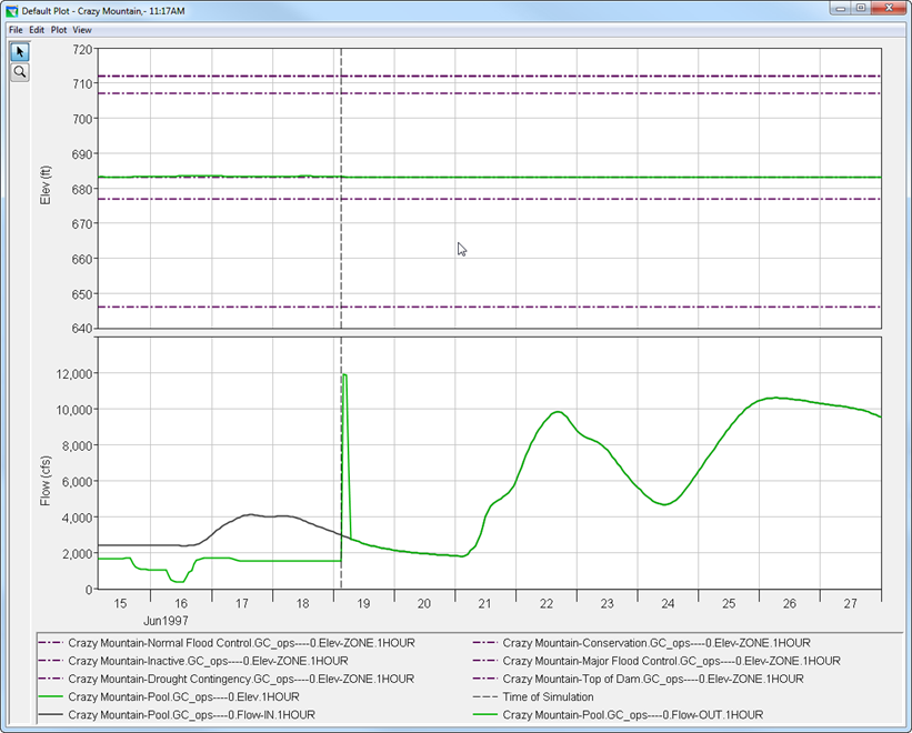
GC_ops alternative – Reservoir Plot
Three different alternatives – Reservoir Comparison Plot
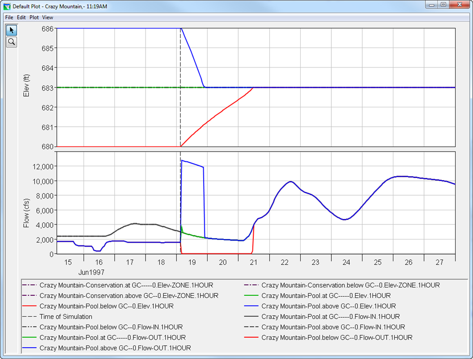
Three different alternatives – Reservoir Comparison Plot

**Bonus Task
- Once the tasks of this workshop are completed, go to the Simulation module, then preview and experiment with a predefined User Report “Workshop_#2_Report”.
- Access this report by first setting Active one alternative at a time, then launching the “Workshop_#2_Report” from the Simulation Module’s Reports>User’s Reports menu.
Question V
At the start of the simulation (19Jun1997 03:00), what is the active reservoir zone? What is the percent storage encroached/filled in that zone?
- GC Ops:
- at GC:
- below GC:
- above GC:
- GC_Ops: Normal Flood Control zone is 0.62% encroached.
- at GC: Conservation zone is 100% filled. Normal Flood Control is 0.00% filled.
- below GC: Conservation zone is 36.39% filled
- above GC: Normal Flood Control zone is 5.16% encroached.
- Edit “Workshop_#2_Report” from the Simulation Module’s Reports menu, and experiment as you wish with modifications to this User Report, for example:
- Modify/Personalize Report Header/Footer: Change text/font/size.
- Edit Contents: Insert/delete/hide columns; create a column that performs calculations.