Workshop 1 – Simple Yield Analysis

WS1_Unsolved.7z

WS1_Solution.7z

Fact Sheet

LAKE TED HILLYER

Reservoir Information

Location: On the Purple River above the confluence with the Orange River.  

Purpose: Water Supply, Flood Control

Lake Data: Based on current sedimentation survey

Model Information

Networks

1. Basic Network – Contains a single reservoir (Upper)

Operations Sets

1. Basic Min Release – Simple minimum release

Rules

1. Min Release – Specifies a constant release year-round in all zones for water supply

Alternatives

1. Basic – Standard run with inflow time series only

Simulations

1. Full Period – Runs the full historical period (1943 – 1993)

Workshop #1 – Simple Yield Analysis

Part 1.a – Sequent Peak Method

• Open the Excel spreadsheet saved as …\Workshop1\Workshop #1.xlsx
• This spreadsheet contains a pre-populated example of the sequent peak method calculations and plots on the "Sequent Peak Method" sheet.
• The monthly average inflow to a reservoir is stored in column B.

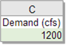
• A hypothetical demand for water supply is defined in Cell C2. This demand is applied to every month in the period of record (1943 – 1993).
• Columns D and E convert the inflow and demand from flow (cfs) to volume (1000 acre-feet [KAF]).
• Columns F and G calculate the accumulated net inflow each month. The net inflow is defined as the gross inflow (column D) minus the demand (column E).
• Columns H and I calculate the accumulated shortage each month. Shortage occurs when the inflow in a month is less than the demand. The accumulated shortage can never be less than zero. If the inflow is larger than the demand for multiple months in a row, the reservoir has surplus water, and the shortage is set to zero.
• The chart to the right of the data table shows the two accumulated time series together, Net Inflow (blue) on the left axis, and Shortage (pink) on the right.
• The storage required to meet the input demand can be determined in two ways:
  • The accumulated net inflow time series (blue) can be examined to find the largest drop between a peak and the subsequent trough. The difference between the peak and trough is the required storage.
  • The accumulated shortage can also be used. The largest accumulated shortage across the full period is the required storage.
  • The results of these two methods are the same.
• Play with the demand by changing the value in Cell C2. See what happens on the plot when the demand changes. Pay attention to the scales on both vertical axes, they will change to fit the data as the demand changes.
  • What happens if the demand decreases? Does the required storage increase or decrease? How much? Is the critical period the same?

• •  What happens if the demand increases? Does the required storage increase or decrease? How much? Is the critical period the same?  What is the upper bound on demand?

• • What happens if the demand is set to a higher flow than the long-term average inflow (2081 cfs)? Can this demand be met? What happens to the accumulated net inflow? Are the results of this calculation still valid in this scenario?

•  Results
  • Determine the required storage for a demand of 1000 cfs. What is the critical period for this demand?

• • Determine the required storage for a demand of 1800 cfs. What is the critical period for this demand?

Part 1.b – Rippl Method (time permitting)

• In the same spreadsheet, the "Rippl Method" sheet contains an example of the same analysis done using the Ripple Method.
• The plot shows the accumulated inflow (note this is now the total inflow, not net inflow as in part 1) and a demand line with a slope matching the demand input in Cell C2. The plot is zoomed into the first drought in the period.
• The required storage to meet the demand is found as the largest vertical distance between the accumulated inflow and the demand line.
• The starting date for the demand line may need to be changed to ensure it is tangent to the accumulated inflow at the beginning of the critical period. You can change the date in Cell G6 to set where the demand line begins.
• Try some of the same demands you used in part 1 of this workshop. Change the start date for the demand line accordingly, and try to measure the required storage as the maximum distance between the two lines (the demand line should be above the inflow line). Do you get the same results?

Part 2 – Iterative Simulation

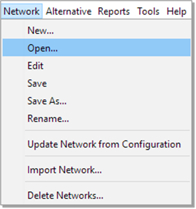
• Open the HEC-ResSim watershed stored in …\Workshop1\Workshop1.wksp
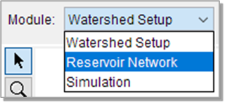
• Go to the Watershed Setup Ensure that the ‘One Res’ configuration is selected.

• Examine the layout of this watershed. There are two rivers and (for now) a single reservoir. There are a number of computation points downstream of the reservoir. This basic layout will be used for all of the HEC-ResSim tasks in this course.

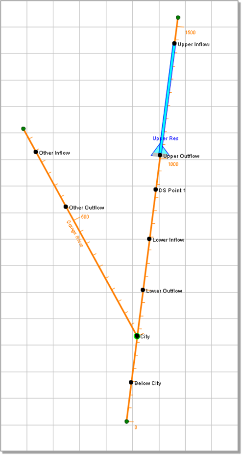
• Go to the Reservoir Network Open the ‘Basic Network’ network.

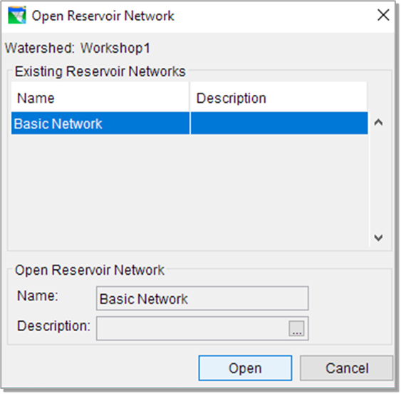
           Notice that the computation points downstream of the reservoir are not included in this network. They are not needed yet.

• Open the Reservoir Editor for ‘Upper Res’ by double clicking on the reservoir. Go to the Physical tab.

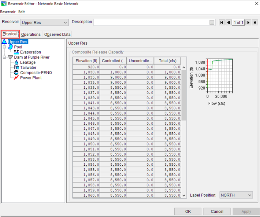
• Examine all the physical components of this reservoir.
  • Look at the elevation-storage-area relationships under Pool. How much water can this reservoir hold? How big is the water surface when completely full?

• • Look at the Evaporation. This workshop is setup with zero evaporation each month. Think about how the yield and required storage might change if evaporation is included.

           NOTE: Evaporation is a critical input to a water supply study and can have significant effects on the result. We are ignoring evaporation for this workshop to focus on the mechanics of firm yield analysis but will include evaporation in later workshops.            

• • There is a Leakage component on the dam, but the leakage is zero for this workshop.
  • Tailwater stage is defined using a simple rating curve. Tailwater stage is used in calculating hydropower production.
  • There is a single controlled outlet named Composite-PENQ. This outlet represents the composite capacity of all available non-turbine outlets on the reservoir. For our modeling, there is no need to specify individual outlet capacities. Some studies may require this.
  • A Power Plant is also defined. The outlet capacity is dependent on the reservoir elevation and is not a monotonic function. Capacity decreases at high heads, as is common with turbines.
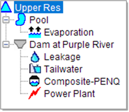
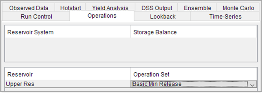
• Go to the Operations tab.  We have one operation set defined so far. The reservoir is split into 5 elevation zones, each with a constant year-round top elevation. The zones are shown graphically on the right side of the tab. In the list on the left side of the tab, Conservation and Inactive zones are formatted differently than the rest. HEC-ResSim considers these zones special.

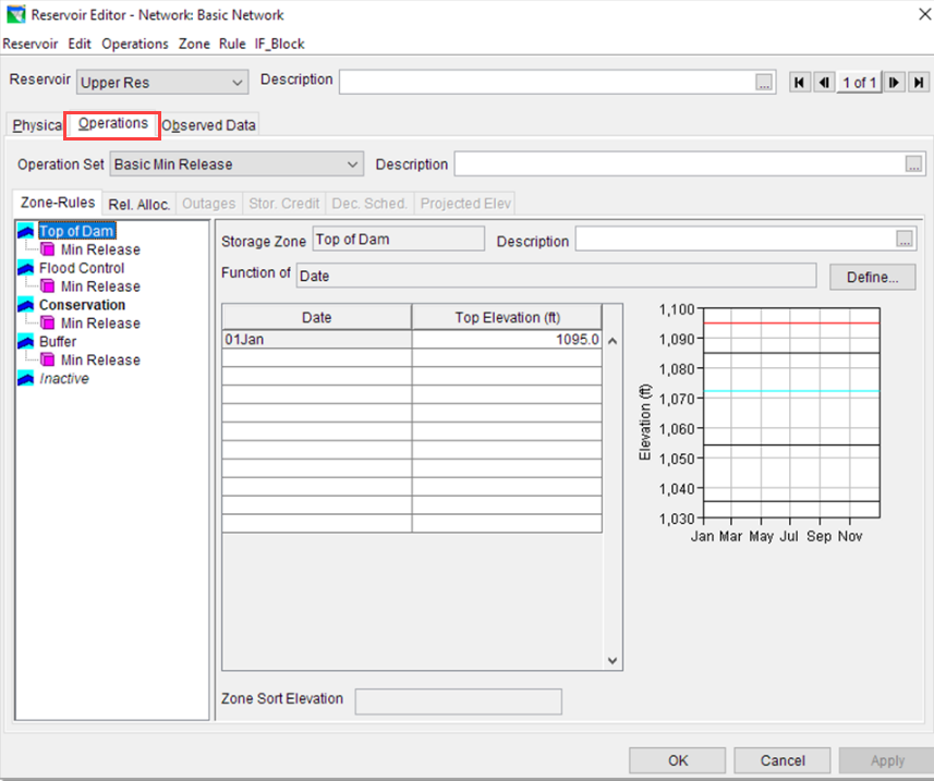
• • The Conservation zone is bold, indicating it is set as the Guide Curve for the reservoir.
    • The model will attempt to keep the simulated storage equal to the guide curve at all times, unless a rule or physical capacity limit prevents it.

• • The Inactive zone is italic, indicating it is set as the Inactive pool for the reservoir.
    • The Inactive zone cannot contain rules, as no operations are possible when the reservoir is that low.

• There is one rule in each zone, except for the Inactive zone. The same rule is used in each zone, and changes made to one copy will apply to all the others. The ‘Min Release’ rule specifies a minimum release in each timestep. This rule corresponds to the demand from the spreadsheet example. The initial demand value is 1000 cfs.
• Close the Reservoir Editor.
• Open the Junction Editor and look at the ‘Upper Inflow’ junction.

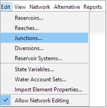
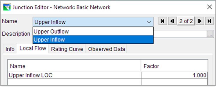
            Note that there is a local inflow defined at this junction with the name “Upper Inflow LOC”.

• Close the Junction Editor.
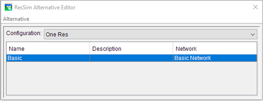
• Open the Alternative Editor.

• • Select the ‘One Res’ configuration and the ‘Basic Network’ alternative.

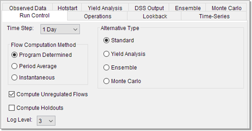
• • On the Run Control tab, see the simulation timestep and the Alternative Type. While many water supply studies may only require monthly analysis, HEC-ResSim runs at daily or smaller timesteps. Daily is short enough for this study. Make sure the Alternative Type is set to Standard, for now. We will explore the Yield Analysis type later. Make sure that the Compute Unregulated Flows box is checked and the Compute Holdouts box is unchecked. Set the Log Level to 3.

• • On the Operations tab, note that the operations set we looked at earlier is selected.

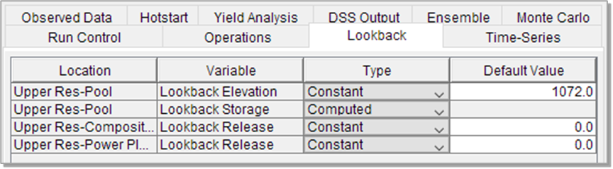
• • The Lookback tab specifies starting values for different model time series. These values are not critical, as long as they are set to a reasonable value. If in doubt, set the Lookback Elevation to the guide curve, and the Lookback Releases to zero.

• • The Time Series tab maps the needed inputs to time series saved in a separate HEC-DSS file. Our simple model has only one input for now – the inflow at the upstream end of the reservoir. This is the same inflow we saw in the sequent peak spreadsheet.

• Close the Alternative Editor.
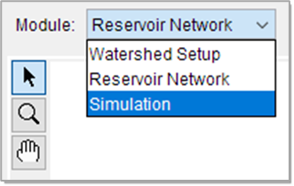
• Go to the Simulation Module.

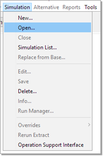
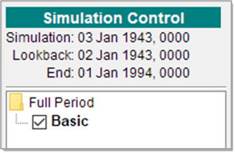
• Open the ‘Full Period’ simulation.

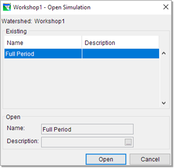
• Note the period of record for this simulation. Note the one included Alternative. Make sure the ‘Basic’ alternative is active and checked.

• Run the simulation.

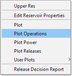
• Several built-in plots are available by right clicking on the reservoir. The Plot Operations plot will be useful for this workshop, as it shows storage by default. Feel free to look at the other plots as well.
• Open the Plot Operations plot.  Note the storage on the top subplot. How low does it get with the initial demand of 1000 cfs? Is it close to the bottom of the conservation zone (which is the top of the inactive zone)?

• Note how the minimum release of 1,000 cfs from our rule prevents the model from releasing less than that value at any point in the record. Note how the physical outlet capacities we defined also limit the release, and force the reservoir to store water in the flood control zone occasionally.
• How does the size of the conservation zone (reference the project fact sheet) compare to the required storages we saw in part 1?           

• Change the minimum release to 1800 cfs by right-clicking the reservoir and selecting Edit Reservoir Properties. Change the value in the minimum release rule, then click OK or Apply to save your changes. Re-run the simulation. What happens to the simulated storage? Are we able to meet this demand with the available storage?           

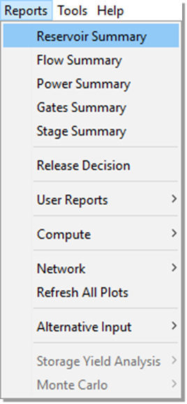
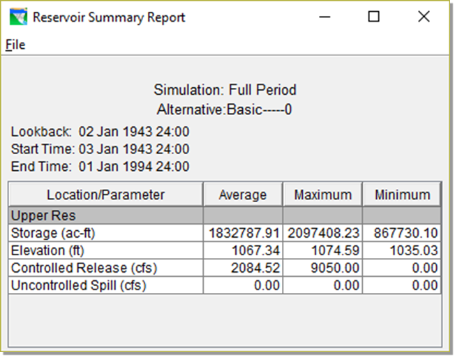
• Try to figure out the firm yield of the conservation pool as it is currently modeled. Change the minimum release until the release is able to be met at all times, while drafting the simulated storage down to the bottom of the conservation pool. The Plot Operations plot can be used to visualize the results to help with this task. Also, the Reservoir Summary Report can be used to see the minimum pool elevation and storage during the run.

• • What is the actual minimum release during your full period of record? Is it the same as the minimum release you specified in your rule?                     

• • What is the minimum storage reached in the period? How close it is to the bottom of the conservation pool?

• • What is the critical period for this reservoir?

• Go back to your spreadsheet from Part 1 of this workshop. Use the firm yield you found in step 20 above as the demand in the spreadsheet. What required storage do you get? Does it match the size of the conservation zone in the HEC-ResSim model? Why or why not?