Workshop 2 – HEC-ResSim Yield Analysis Tool

WS2_Unsolved.7z

WS2_Solution.7z

Fact Sheet

LAKE TED HILLYER

Reservoir Information

Location: On the Purple River above the confluence with the Orange River.  

Purpose: Water Supply, Flood Control

Lake Data: Based on current sedimentation survey

Model Information

Networks

1. Basic Network – Contains a single reservoir (Upper)

Operations Sets

1. Basic Min Release – Simple minimum release
2. Varying GC – Higher summer pool elevation than basic
3. Varying GC 2 – Higher summer pool, lower winter pool than basic
4. Varying Demand – Flat guide curve, seasonally-varying demand

Rules

1. Min Release [operations] – One for each operation set

Alternatives

1. [operations] – One for each operation set, Yield Analysis runs

Simulations

1. Full Period – Runs the full historical period (1943 – 1993)

Workshop #2 – HEC-ResSim Yield Analysis Tool

Yield Analysis with a constant guide curve

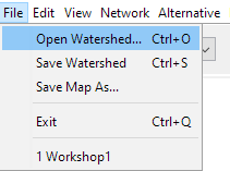
• In HEC-ResSim open the watershed saved as …\Workshop2\Workshop2.wksp

• This watershed is similar to what we used in Workshop #1, but with some different options included.
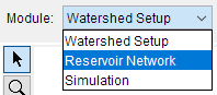
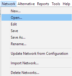
• On the Reservoir Network module, open the network named 'Basic Network'.

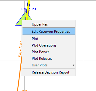
• Open the Reservoir Editor for 'Upper Res'. Note that the physical parameters are identical to Workshop #1.
• Go to the Operations tab. Note that we now have four operations set.

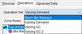
• • The Basic Min Release operations set is the same as in Workshop #1, with a constant guide curve.

• • The Varying Demand operations set has the same constant guide curve as the Basic Min Release set but has a seasonally varying demand. We will use this set to look at the impacts of this seasonal demand variation on firm yield.
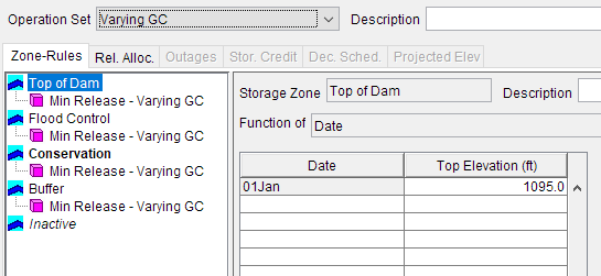
  • The Varying GC operations set is similar, but with a guide curve that varies across the year. Open this operations set and examine the Conservation zone. Note the changes to the zone top elevation.

• • The Varying GC 2 operations set has a different curve variation than the last set. This will be used to show the impact of different changes on the resulting firm yield.
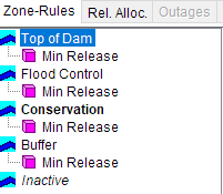
  • Note that the different operations sets can share rules. Changes made to a rule in one set will apply to any other sets that rule is in. Here we use a different rule in each set to avoid unintentionally making changes to other sets.

• Open the Alternative Editor. Ensure the 'Study' configuration is selected.

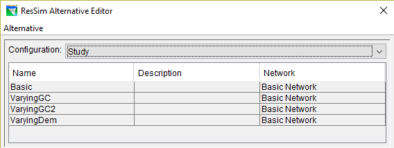
• See the four defined alternatives, matching the operations sets we saw earlier. Flip between the alternatives while browsing the different tabs to see similarities and differences.
  • On the Run Control tab, note the Alternative Type. We have changed from Standard in the last workshop to Yield Analysis in this one. This will allow us to use the new features of HEC-ResSim to automate some of the work from Workshop #1.
  • On the Operations tab, note that each alternative has a different operations set selected. This is the primary difference between each of the three alternatives. Changing the alternative while keeping the network the same will allow us to run each alternative quickly in the Simulation module.
  • The Time-Series and Lookback tabs include the same starting values and the same inflow time series as in Workshop #1, with the lookback pool elevation changed to match the top of the conservation pool in each operations set.

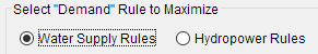
• • The Yield Analysis tab is now usable since we selected Yield Analysis as our alternative type.
    • We can run our analysis on water supply or hydropower. Select Water Supply Rules for this workshop.

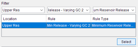
• • • The yield analysis tool works similarly to what we did in Workshop #1. It will change the minimum release on a rule until the minimum can be met at all times while also drafting the storage to the bottom of the conservation pool. This means we have to choose a rule for the tool to modify. The rule needs to be a minimum constraint. We only have one rule in each operations set. Select the relevant rule on each alternative.

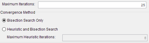
• • • The tolerances can be changed if convergence is taking too long, or we need more precision. Leave the default values for now.

• • • We can also adjust the iteration parameters to limit the number of iterations and try using the heuristic search. Use 25 iterations and the Bisection Search Only.

• • • Make sure all three alternatives are setup the same way. Since we used different water supply rules for each operations set, we must select the correct rule in the Yield Analysis tab for each alternative.
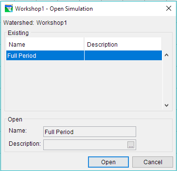
• Go to the Simulation Module and open the 'Full Period' simulation. You can see that this simulation includes all four of the defined alternatives.

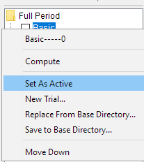
• Set the 'Basic' alternative as active by right clicking on the 'Basic' alternative in your Simulation Control window. The alternative that is set as active will be bolded.

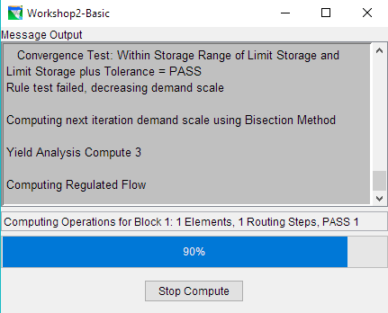
•  Run the simulation. This run will take a bit longer, as the yield analysis tool iterates towards a solution. The Compute window will show the details of the iteration as it runs.
  
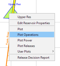
• • Open the Plot Operations plot on 'Upper Res' by right clicking on the reservoir and selecting Plot Operations. Does the storage draft down to the Inactive zone once in the period? How long does the storage stay at the bottom limit?

Please note that built-in Yield Analysis plots are planned as a future enhancement to HEC-ResSim.

• • Open the Reservoir Editor for 'Upper Res'. What release did the yield analysis tool end up with (look at the value set in the minimum release rule)? How does that compare with the yield you calculated in Workshop #1? Is the critical period the same or different?

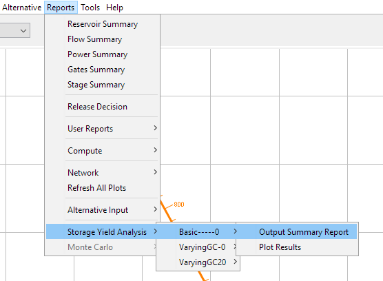
• • Open the Storage Yield Analysis Output Summary Report for this alternative. This report shows the iteration details from the latest run.

• • • The Demand Estimate Factors show the factor used to scale the initial demand up or down. The range of possible factors should get smaller as the iterations progress.
    • The Min Release Average Annual Demand (cfs) shows the actual release set on the rule for each iteration (or the average annual release for varying demands).
    • The Storage Convergence shows the progress towards drafting the storage completely during the run.
    • The Flow Convergence shows progress towards ensuring that the minimum release is always met.
    • How many iterations were required to converge (starting with an initial release of 1000 cfs)? What might happen if you changed the flow or storage tolerances?

• Run the 'VaryingGC' alternative. This alternative has the guide curve 8 ft higher in the summer compared to the 'Basic' alternative. The winter guide curve is the same. For this and the following alternative runs, plot the results vs. the basic run by checking the current alternative and the basic alternative names in the Simulation Control window on the right, then opening your plot by right-clicking on the reservoir. This will plot results from all checked alternatives.
  • What is the yield for this alternative?

• • What is the critical period?

• • How did the extra summer storage affect the yield?

• Run the 'VaryingGC2' alternative and consider the same questions.
  • How does lowering the winter pool affect the yield?

• • Does the higher summer pool provide enough extra storage to balance the lost winter storage?

• Now run the 'VaryingDem' alternative. Remember that as the yield analysis tool iterates, it will scale the demand up and down while keeping the same seasonal pattern.
  • What effect does the seasonal demand have on the firm yield?

• • The initial demand was 800 cfs in the winter and 1200 cfs in the summer. Are the final winter and summer demands still 400 cfs apart? Why?

• • Look at the Storage Yield Analysis Output Summary Report for this run. How does the report list the demand used in each iteration?

• • If you have extra time, try changing the guide curve elevations in the VaryingGC2 alternative to result in a similar yield to the constant guide curve we started with. Use a constant annual demand. Which factor seems to be more sensitive, the summer elevation or the winter elevation? What does that tell you about this reservoir?