Workshop 3 – Data Requirements

WS3_Unsolved.7z

WS3_Solution.7z

Fact Sheet

LAKE TED HILLYER

Reservoir Information

Location: On the Purple River above the confluence with the Orange River.  

Purpose: Water Supply, Flood Control

Lake Data: Based on current sedimentation survey

Model Information

Networks

1. Basic Network – Contains a single reservoir (Upper)

Operations Sets

1. Basic Min Release – Simple minimum release

Rules

1. Min Release – Year-round minimum release for water supply

Alternatives

1. Basic – Yield Analysis run with min release operations

Simulations

1. Full Period – Runs the initial full historical period (1943 – 1993)

Workshop #3 – Data Requirements

In this workshop you will include evaporation in your model and adjust the inflow to the reservoir accordingly. You will evaluate the effects of including evaporation on the resulting firm yield. Next you will extend the inflow time series to include more recent years of data. You will process these extended inflows to remove evaporation and then evaluate the firm yield again using the longer data set.

Part 1 – Adding Evaporation to the Simulation

• In HEC-ResSim open the watershed saved as …\Workshop3\Workshop3.wksp
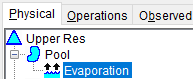
• Add an evaporation time series to the model. Navigate to the Evaporation element on 'Upper Res'.
  • On the Reservoir Network module, open the network named 'Basic Network'.
  • Open the Reservoir Editor for 'Upper Res'.
  • Go to the Physical tab.
  • Select Evaporation.

• • Select the Evaporation Time Series option near the bottom of the Reservoir Editor window.
  • Click Apply and close the editor.
• Open the Alternative Editor and choose the 'Basic' alternative.
• Go to the Time-Series tab. A new row has been added to the table because you told HEC-ResSim you wanted to use an evaporation time series.
  • Fill in the pathname for the evaporation time series. A time series of net evaporation (evaporation minus precipitation) has been provided in the workshop folder.
  • Make sure the empty table row is selected and click the Select DSS Path… button.

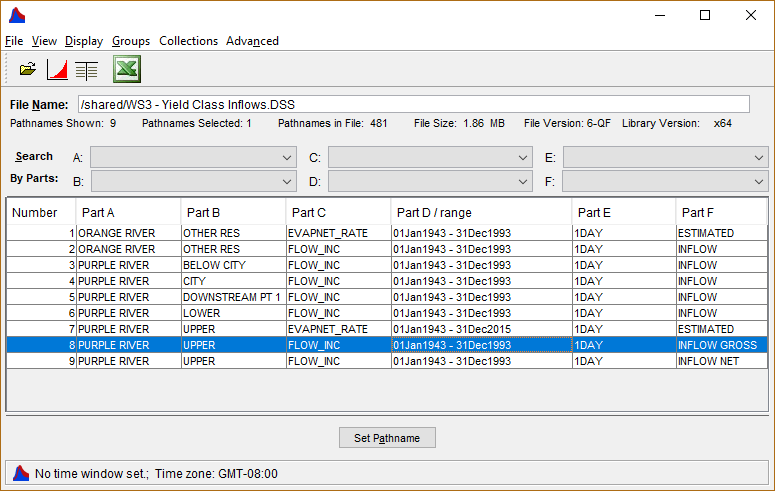
• • In the HEC-DSSVue window that appears, click the Open symbol, navigate to the 'shared' directory, and select 'WS3 - Yield Class Inflows.DSS'

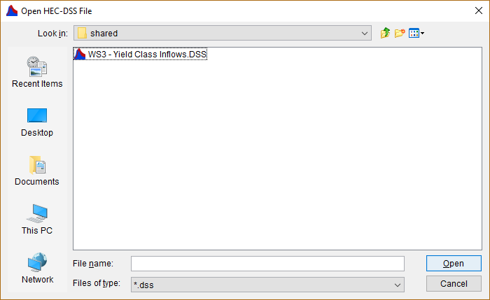
• • Select '/PURPLE RIVER/UPPER/EVAPNET_RATE//1DAY/ESTIMATED/'. Click Set Pathname and close the window.

• • The blank table row should now be filled in with the name and location of the evaporation time series.
• Review the settings in the Yield Analysis tab. Make sure that the selected options make sense and that the correct rule is selected.
• Now your model is subtracting the net evaporation from the reservoir storage every time step. Do you think this will increase or decrease the firm yield of the reservoir?

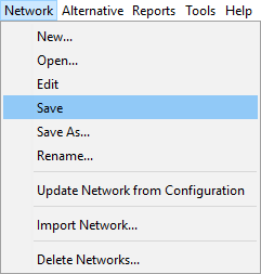
• Save your alternative and close the Alternative Editor. Save the Network to retain the change you made to 'Upper Res'.

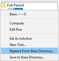
• Switch to the Simulation module. Open the 'Full Period' simulation which will run the 'Basic' alternative for the same period as in the last workshop. Remember that every simulation is a separate copy of the model, so the changes you just made do not show up yet. Right click on the 'Basic' alternative on the right side of the HEC-ResSim window and select Replace From Base Directory… This will update the simulation with the latest version of the 'Basic' alternative, including changes to the network.

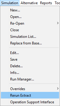
• Because you added a time series, this copy of the model will not have the time series you just pointed to yet. You must extract the time series from the original DSS file into the simulation dss file. Do this by selecting the Rerun Extract option in the Simulation menu.

• Run the simulation (including Yield Analysis) again. What firm yield do you calculate now?

• You know from the lecture that if you model evaporation from the reservoir surface, you need to adjust the inflow to not include evaporation. Currently your model is double-counting evap by removing it explicitly while also using an inflow time series that is net of evaporation. You need to update the inflow to be the flow before water is lost to evap. This inflow has already been calculated and stored in the DSS file. Open the Alternative Editor (either here or back in the Network module, your choice). Change the 'Upper Inflow LOC' time series by choosing '/PURPLE RIVER/UPPER/FLOW_INC//1DAY/INFLOW GROSS/' from the same DSS file you used for the evaporation time series.

• If you changed the alternative in the Network module, remember to save your change and update the copy in the simulation.
• In the Simulation module, re-run the extract again to pull in the new inflow time series.
• Re-run the yield analysis. What do you get for firm yield?

• You have correctly accounted for evaporation separately from the inflow. Now you can evaluate revisions to the reservoir and operations that change the pool elevation and surface area away from their historical values while still calculating an accurate evaporation amount and firm yield.
• What would happen if you used total evaporation (actual evaporation from the reservoir surface) instead of net evaporation (total evaporation minus the precipitation falling on the reservoir surface)?

• What if you simulated using gross inflow, but did not include evaporation losses in the simulation?

Part 2 – Record Extension

You will practice some data manipulation now by extending the period of record by 22 years. This is similar to what you might need to do if you were updating an older yield study with more recent data.

• Open the Excel spreadsheet at: '\Workshop3\Record Extension Data.xlsx'
• Go to the 'Mass Balance' sheet. This sheet contains pool elevation (Column B) and outflow (Column C) time series for 1994 – 2015, to extend the original period that ends in 1993.
  • The sheet also has a copy of the same elevation-storage curve present in the HEC-ResSim model in Columns J and K.
  • Pool elevation has been converted to storage using the curve, linearly interpolating between the closest two elevations. Results are available in Column E. The lack of a built-in interpolation function in Excel requires the use of complicated-looking OFFSET() functions, the purpose of which is to interpolate between the closest two pool elevation values for each timestep.
  • The change in storage each day (Storaget-Storaget-1) is calculated in acre-feet in Column F and converted to cfs in Column G.
  • In Column H, calculate inflow (net of evaporation losses and precipitation gains) using the mass balance equation presented in the lecture.

                     Inflowt=Storaget-Storaget-1+Outflowt

• • Because calculating a change requires 2 values, we cannot calculate the change in storage for Jan 1, 1994 easily in this spreadsheet, and therefore cannot calculate an accurate inflow for that day. You can either manually calculate that day using the pool elevation for 31 Dec, 1993 or leave it blank for now and approximate the inflow later.

                   The chart will update to show the net inflows on top of the outflows. Notice how the inflows are a more "natural" looking flow with seasonal ups and downs, whereas the outflow has no consistent seasonal pattern but does have a clearly defined minimum around 500 cfs. Also note that the calculated inflow has some noise. This is                              normal in calculated inflows, due to small errors in measurements of pool and outflow.

• Now adjust those net inflows to remove evaporation. Go to the 'Evaporation' sheet. Here you will use daily evaporation to adjust your inflows.
  • The observed pool elevation (Column B) and the net inflow (Column C) you just calculated are populated from the first sheet.
  • Evaporation depth estimates are in Column D. These values are net evaporation, or evaporation minus precipitation, which can be negative in wetter months. Note that each day in a given month has the same evaporation, indicating this data was likely estimated using monthly sums and disaggregated to a daily timestep.
  • The elevation-area curve from the HEC-ResSim model is stored in Columns K and L.
  • Column F converts each elevation value to an equivalent surface area by linearly interpolating on the Elevation-Area curve.
  • Column G multiplies the surface area for that day by the evaporation depth to get evaporated volume in acre-inches/day, then divides by 12 to get ac-ft.
  • Column H then converts from ac-ft/day to cfs. Now each daily evaporation volume value in a month is different because the identical evaporation depths are multiplied by a varying surface area.
  • Calculate a gross inflow in Column I that represents flow into the reservoir before evaporation and precipitation on the reservoir surface occur.

                     Gross Inflow=ΔStorage+Outflow+Losses=Net Inflow+Losses

• Save your work.
• Now you need to import your calculated gross inflow to the HEC-DSS file so you can use it in your HEC-ResSim model. Open '\Workshop3\shared\WS3 - Yield Class Inflows.DSS'. HEC-DSSVue has utilities to import data from Excel, but for a single time series a manual import will work. You can also access HEC-DSSVue from the Tools menu in HEC-ResSim.
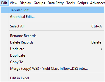
  • There is already a gross inflow time series that has data from 1943 – 1993. Add data to the end of this time series through the Tabular Edit… option on the Edit menu.

• • Copy all the gross inflow data in your spreadsheet for 1994 – 2015 and paste into the Edit window of HEC-DSSVue. Select the empty cell for 01 or 02 Jan 1994 24:00 at the bottom of the Manual Entry tab and paste. This will extend the data through 2015.

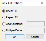
• • If your 01 Jan value is blank, you can use HEC-DSSVue to interpolate between the days to either side. Select the three days from 31 Dec, 1993 to 02 Jan, 1994 and right click and select Fill… Then select Linear Fill and hit OK. This will interpolate linearly and fill in any selected blank values.

• • Click Save and then No on the popup window that asks if you want to return to the data entry screen. Your inflow time series is now extended.

• Go back to the Workshop3 HEC-ResSim watershed.
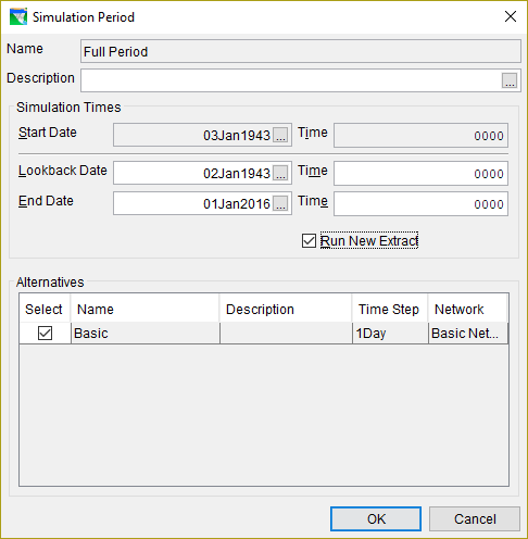
• Open the 'Full Period' simulation, then edit it. To extend the run period, change the End Date from 01Jan1994 to 01Jan2016. Note that the time is 0000, which is equivalent to 2400 on December 31, 2015. Check the Run New Extract box to ensure that the extended data is brought into the simulation.

• Run the Yield Analysis again using the extended period. What firm yield do you calculate now? What is the critical period?

• Does calculating a different firm yield now mean that the original firm yield you found was wrong? Why?

• What are some broader implications of this new critical drought? Does this mean that other projects in the same river basin or region will also have a new critical drought?

• OPTIONAL: If you have extra time, experiment with changing the simulation dates more. Move the end date earlier, or the start date later (this requires creating a new simulation, as start dates cannot be edited). Try starting and ending in different parts of the hydrologic cycle. Does this impact the firm yield? Why?

• OPTIONAL: We have been using daily average inflows so far. What might change if we were using monthly average values instead? Convert your gross inflow time series to monthly using the Tools → Math Functions… → Time Functions → Change Time Interval tool. Notice how the inflows are now constant each month at the monthly average flow. Use this time series in the model instead. HEC-ResSim will automatically convert to daily for you with each day's value equal to the average flow for that month. How does this change your firm yield estimate? Is monthly data more or less conservative than using daily data?

• OPTIONAL: A time series with some data problems is provided in the HEC-DSS file as '/PURPLE RIVER/UPPER/FLOW_INC//1DAY/INFLOW EXT GROSS ERRORS/'. Look through this time series and identify any obvious errors or suspect values. It can help to plot the time series and zoom in on suspect periods or tabulate and scroll to the suspect periods. What could have caused these problems? How might you fix them?