Workshop 7 – Reliability and Uncertainty

WS7_Unsolved.7z

WS7_Solution.7z

spreadsheet:  Ensemble Results.xlsx

Fact sheet

LAKE TED HILLYER

Reservoir Information

Location: On the Purple River above the confluence with the Orange River.  

Purpose: Water Supply, Flood Control

Lake Data: Based on current sedimentation survey

Model Information

Networks

1. Basic Network – Contains a single reservoir (Upper)

Operations Sets

1. Basic Min Release – Minimum releases for water supply

Rules

1. Min Diversion – Constant year-round release through dam

Alternatives

1. Basic – Yield Analysis (reservoir) run using Basic network and Basic water account set
2. Ensemble – Yield Analysis (reservoir) run using a single ensemble trace of synthetic hydrology

Simulations

1. Full Period – Runs the initial historical period (1943 – 1993)
2. EnsemblePeriod – Runs the synthetic hydrology period (2101 – 2200)

Workshop #7 – Reliability and Uncertainty

In this workshop you will work in groups to investigate the uncertainty in the basic firm yield analysis you have done previously. You will also run stochasticly generated inflows through the model to calculate reliability metrics. Results from each group will be combined and we will go over them as a class.

Part 1 – "Lifetime" Reliability

• In HEC-ResSim open the watershed saved as '\Workshop7\Workshop7.wksp'
• In Workshop #2 you calculated a firm yield near 1535 cfs for a scenario with no explicitly modeled evaporation or water accounts and only a single water supply rule. Now you will use an ensemble of inflow time series to evaluate other possible yields for the same scenario. The inflow traces in the ensemble were created using an autoregression model with parameters based on the original period of record observed values. Each trace represents a possible future hydrology with statistical characteristics similar to the observed record. These 50 possible hydrologies are each 100 years long, and may each have critical droughts that are more intense or milder than the observed critical drought. The 50 firm yields calculated from these traces will give a fuller picture of the water supply capability of the reservoir.
• You will split into groups for this workshop, and each group will calculate firm yields for some portion of the traces. Afterwards, each group's results will be combined for further analysis as a class.
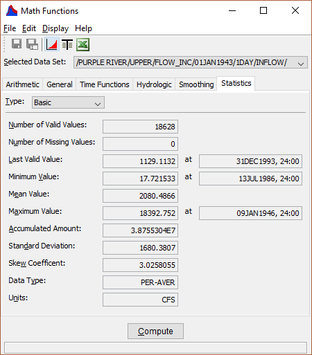
• The ensemble traces are stored in '\Workshop7\shared\StochasticFlowBase.dss'. Open this file now to view it using HEC-DSSVue.
  • Each trace extends for an arbitrary period of January 2101 – December 2200. The traces are numbered 001 – 050 in the F-Part. Plot a few of the traces to get a feel for the magnitude and patterns in the flows. The observed inflows are saved in the same DSS file with an F Part of 'INFLOW'. You can also compare these observed flows to the traces, though the time periods will not be the same. If you want to explore the statistics of the traces, the Tools menu -> Math Functions… -> Statistics tab has many options. Note that the daily inflows have significant variability, and the statistics show this. More meaningful statistics could be calculated using monthly or annual inflows, if you would like. Use the Change Time Interval operator in the Time Functions tab in the math functions to convert to longer timesteps if you choose to look at monthly or annual time series. The screenshot below has the historical period inflow daily statistics for your reference.

• Go back to the HEC-ResSim model. The Network is similar to the network from Workshop #2, with a single purpose on the reservoir.
• There are two Alternatives, 'Basic' and 'Ensemble'. These are the same except for the Time-Series input for reservoir inflow. The 'Ensemble' alternative initially points to trace 001 in the DSS file.
• This model has two Simulations saved in it, 'Full Period' (with the 'Basic' alternative loaded) and 'EnsemblePeriod' (with the 'Ensemble' alternative loaded). The 'Full Period' simulation is the same as you have used in previous workshops, while the 'EnsemblePeriod' simulation is set to the same dates as the ensemble traces.
• Your group needs to run the yield analysis for each of your assigned traces. There are several methods you can use to run the traces through the HEC-ResSim model. You could create a new Simulation for each trace and alter the simulation's copy of the 'Ensemble' alternative to read in the correct trace. Or you could use just one simulation but make new Alternatives for each trace. This is the method we will use, as it makes comparing the runs easier.
  • From the Network module, open the Alternative Editor and save the 'Ensemble' alternative as 2 new alternatives: 'Ensemble 2' and 'Ensemble 3'. Then change the inflow for each of these three alternatives to match the three traces you were assigned. (Also, you might need to set the Yield Analysis options, particularly the Selected Demand Rule and the Convergence Method, as HEC-ResSim might not keep these when you copy an alternative.)
  • In the Simulation module, add your new alternatives to the 'EnsemblePeriod' simulation the same way you added an alternative in Workshop #7.
• Run the yield analysis to calculate a firm yield for each of your traces. Quality control the results to ensure the calculation worked as expected. Record each firm yield for later compilation.
• What is the range of the firm yields you calculated?

• How does this range compare to the original yield of 1535 cfs?

• Provide all your yield calculation results to the person compiling the data. Further analysis will be done together as a class.

Part 2 – Annual Reliability

• Now we will look at annual reliability by creating a yield/reliability curve. We will split the work like we did in Part 1. This time, instead of using different ensemble traces, we will just look at trace 001. Each group will calculate the annual reliability of some different demands, and we will compile them together.
• In the Network module, save one of your 'Ensemble' alternatives as 'AnnualReli'. Set the Alternative Type to Standard on the Run Control tab. In this analysis, we want to allow the demand to not be met some of the time, so we can't use the Yield Analysis tool. Set the inflow to use trace 001.
• Add this new alternative to your simulation.
• The firm yield for this trace is 1496 cfs, so that demand will be considered to have 100% annual reliability. Higher demands should have lower reliabilities.
• Run your assigned demands and count the number of years that have a failure. A failure is defined as releasing less than the desired demand at any point in the year. The annual reliability is then 1 – (# of failures / 100), because there are 100 total years of data. We will use calendar years here for ease of counting, but note that water years may be more appropriate depending on the hydrology of a particular study.
  • One way to count failures is to plot the reservoir outflow and visually count the years with outflow below demand. The built-in plots in HEC-ResSim can be used for this, or you can plot the outflow by itself from HEC-DSSVue.

• • This example plot shows two periods with releases less than demand. You would need to zoom in to tell how many different years are affected.
• Provide your results to the person compiling the data. Further analysis will be done together as a class.