Example 2. Analysis with Low Outliers – Orestimba Creek near Newman, CA
Example 2 illustrates the computation of a peak flow frequency curve using EMA and Bulletin 17C procedures with an annual maximum series comprised of systematic flood peaks when low outliers (a.k.a. Potentially Influential Low Flows, PILFs) are present. For this example, USGS gage 11274500 Orestimba Creek near Newman, CA is used. Orestimba Creek is a tributary to the San Joaquin River, whose 134 sq. mi. drainage area lies on the eastern slope of the Diablo Range section of the Coast Range Mountains of California. The drainage basin has an average basin elevation of approximately 1,550 feet with peak flows usually occurring in late winter. Orestimba Creek is one of the few tributaries in the area to maintain a definite stream channel from the foothills to the San Joaquin River (England, et al., 2018).
The Orestimba Creek near Newman, CA stream gage has an annual peak record consisting of 82 peaks beginning in 1932 and ending in water year 2013. Of the 82 annual peaks, there are 12 years for which the annual peak is 0 cfs, meaning the stream was dry for the entire year. The annual maximum series is plotted in Figure 1 and tabulated in Table 1.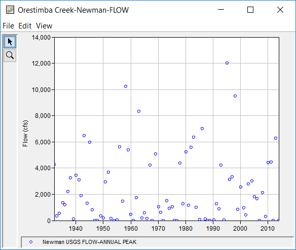
Table 1. Orestimba Creek near Newman, CA Annual Peak Flow Record.
Date | Flow (cfs) |
|---|---|
08 Feb 1932 | 4260 |
29 Jan 1933 | 345 |
01 Jan 1934 | 516 |
08 Apr 1935 | 1320 |
13 Feb 1936 | 1200 |
13 Feb 1937 | 2180 |
11 Feb 1938 | 3230 |
09 Mar 1939 | 115 |
27 Feb 1940 | 3440 |
04 Apr 1941 | 3070 |
24 Jan 1942 | 1880 |
21 Jan 1943 | 6450 |
29 Feb 1944 | 1290 |
02 Feb 1945 | 5970 |
25 Dec 1945 | 782 |
30 Nov 1946 | 0 |
30 Nov 1947 | 0 |
12 Mar 1949 | 335 |
05 Feb 1950 | 175 |
03 Dec 1950 | 2920 |
12 Jan 1952 | 3660 |
07 Dec 1952 | 147 |
30 Nov 1953 | 0 |
19 Jan 1955 | 16 |
23 Dec 1955 | 5620 |
24 Feb 1957 | 1440 |
02 Apr 1958 | 10200 |
16 Feb 1959 | 5380 |
10 Feb 1960 | 448 |
30 Nov 1960 | 0 |
15 Feb 1962 | 1740 |
01 Feb 1963 | 8300 |
22 Jan 1964 | 156 |
06 Jan 1965 | 560 |
30 Dec 1965 | 128 |
24 Jan 1967 | 4200 |
30 Nov 1967 | 0 |
25 Jan 1969 | 5080 |
01 Mar 1970 | 1010 |
21 Dec 1970 | 584 |
30 Nov 1971 | 0 |
11 Feb 1973 | 1510 |
03 Mar 1974 | 922 |
08 Mar 1975 | 1010 |
30 Nov 1975 | 0 |
30 Nov 1976 | 0 |
17 Jan 1978 | 4360 |
21 Feb 1979 | 1270 |
16 Feb 1980 | 5210 |
29 Jan 1981 | 1130 |
05 Jan 1982 | 5550 |
24 Jan 1983 | 6360 |
25 Dec 1983 | 991 |
09 Feb 1985 | 50 |
19 Feb 1986 | 6990 |
06 Mar 1987 | 112 |
30 Nov 1987 | 0 |
30 Nov 1988 | 0 |
28 May 1990 | 4 |
24 Mar 1991 | 1260 |
15 Feb 1992 | 888 |
13 Jan 1993 | 4190 |
20 Feb 1994 | 12 |
10 Mar 1995 | 12000 |
19 Feb 1996 | 3130 |
23 Jan 1997 | 3320 |
03 Feb 1998 | 9470 |
09 Feb 1999 | 833 |
14 Feb 2000 | 2550 |
05 Mar 2001 | 958 |
03 Jan 2002 | 425 |
16 Dec 2002 | 2790 |
25 Feb 2004 | 2990 |
16 Feb 2005 | 1820 |
02 Jan 2006 | 1630 |
30 Nov 2006 | 0 |
25 Jan 2008 | 2110 |
17 Feb 2009 | 310 |
20 Jan 2010 | 4400 |
24 Mar 2011 | 4440 |
30 Nov 2011 | 0 |
24 Dec 2012 | 6250 |
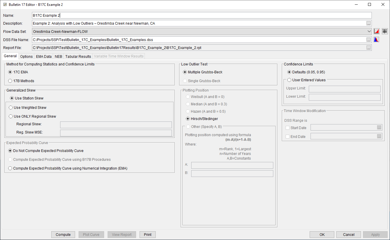
A Bulletin 17 Analysis using EMA and Bulletin 17C procedures has been developed for this example. To open the analysis, either double-click on the analysis labeled "B17C Example 2" from the Study Explorer or from the Analysis menu select open, then select "B17C Example 2" from the list of available analyses. When "B17C Example 2" is selected, the Bulletin 17 analysis editor will appear as shown in Figure 2. As shown, the Skew option was set to use the Station Skew.
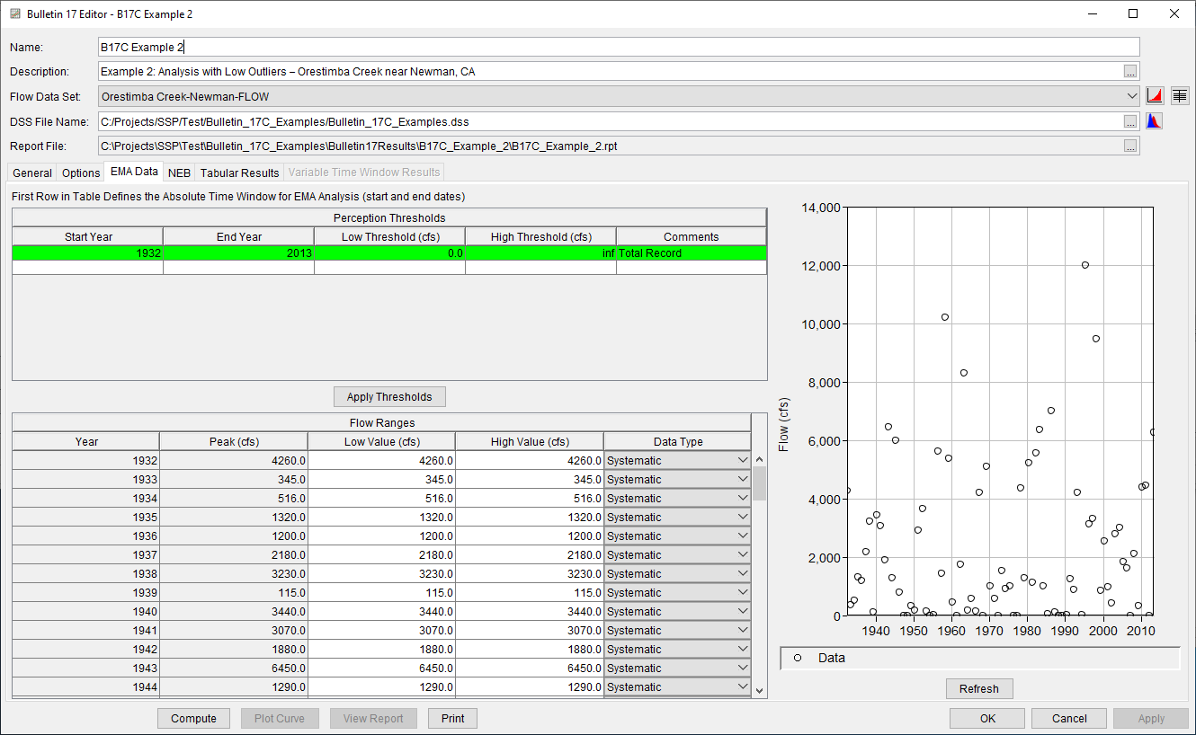
No changes to the Options tab are necessary. The EMA Data tab for this example is shown in Figure 3. Since this example uses an annual maximum series consisting entirely of systematic data with a complete record, a single zero – inf perception threshold is adequate. No modifications to the default flow ranges and data types are necessary.
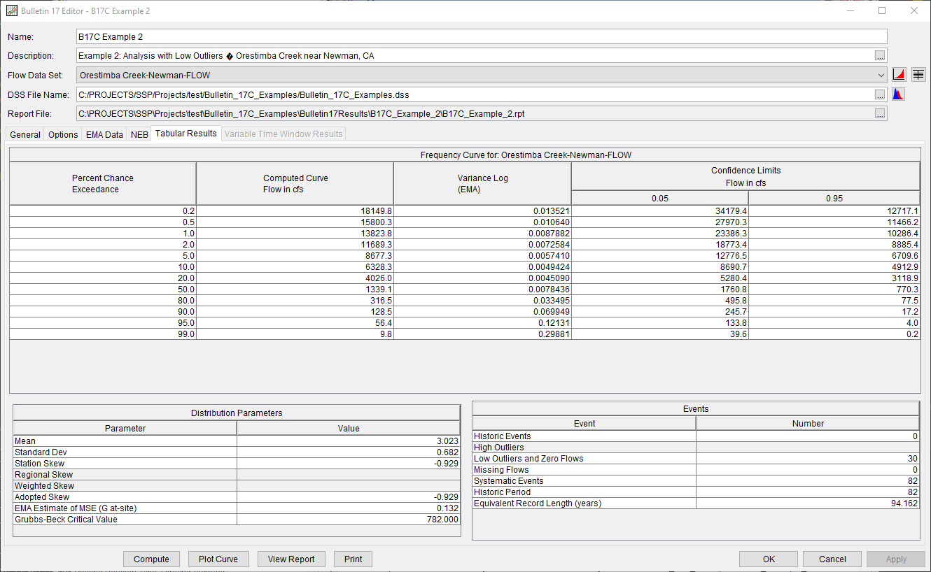
Once all of the General and EMA Data tab settings are set or selected, the user can press the Compute button to perform the analysis. Once the computations have been completed, a message window will open stating Compute Complete. Close this window and then select the Tabular Results tab. The analysis window should resemble Figure 4.
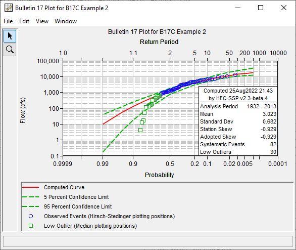
In addition to the tabular results, a graphical plot of the computed frequency curves can be obtained by pressing the Plot Curve button at the bottom of the analysis window. The Log Pearson Type III distribution fit using EMA to the input annual maximum flow data set, the 5% and 95% confidence limits, and the computed plotting positions are shown in Figure 5.
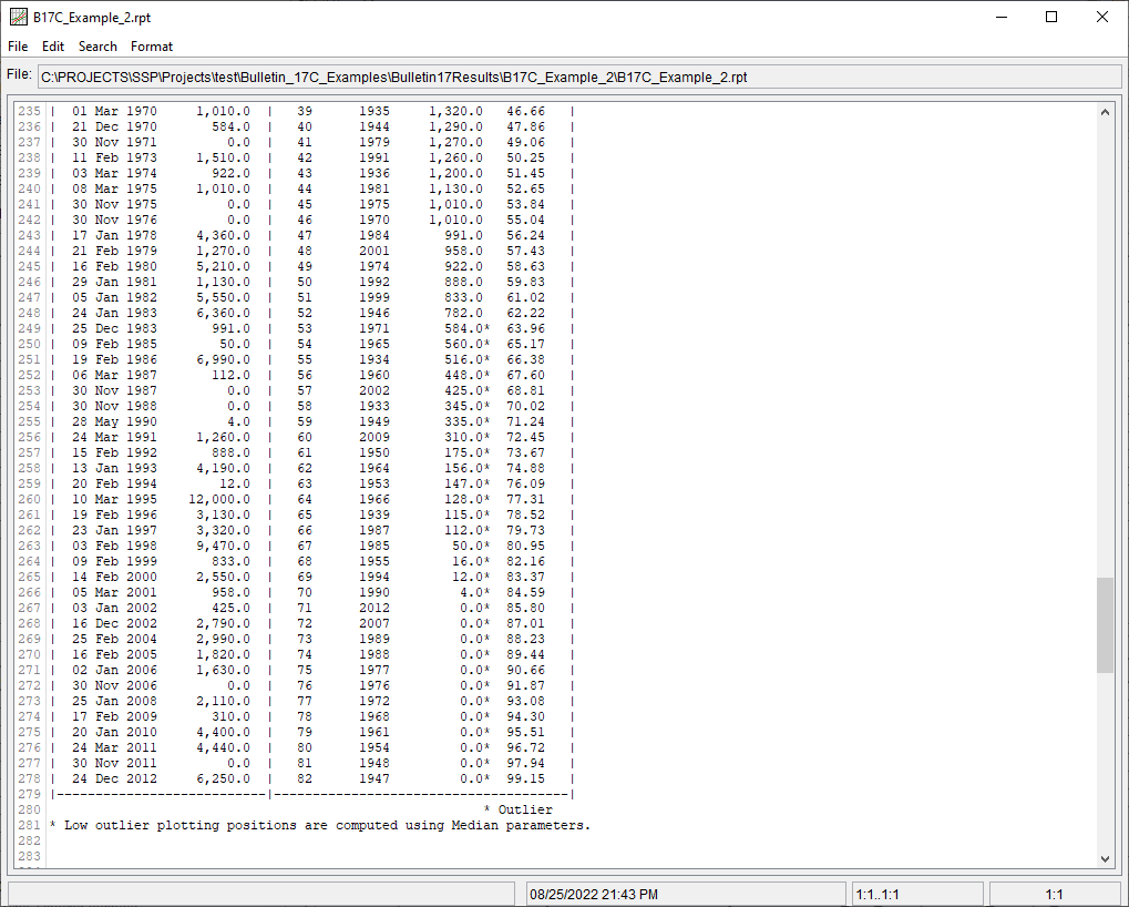
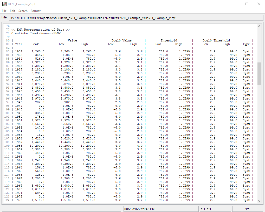
As shown in Figure 4, the Multiple Grubbs-Beck Test identified a low outlier threshold (critical value) of 782 cfs, which corresponds to the smallest peak that was retained. Thirty annual peak flows were thus identified and censored, as shown in Figure 6. These annual peak flows were then recoded to have a flow interval of zero – 782. The perception threshold for all systematic observations were also adjusted to correspond with the Multiple Grubbs-Beck Test low outlier threshold (i.e. 782 – inf), as shown in Figure 7.
