Download PDF
Download page Example 15. Coincident Frequency Analysis, A and B can be Assumed Independent.
Example 15. Coincident Frequency Analysis, A and B can be Assumed Independent
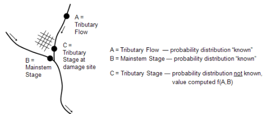
This example demonstrates how to create a coincident frequency analysis. Figure 1 illustrates the scenario for Coincident Freq Test 15. The goal of this example is to develop a stage-frequency curve at a point along the tributary (variable C) given flows on the tributary (variable A) and flows in the mainstem (variable B). Large flows on the mainstem do cause backwater along the tributary and thus affect the stage at the point of interest. The data for this example comes from an existing flow frequency curve for Variable A and an existing flow duration curve for Variable B. An HEC-RAS model was used to simulate the response of Variable C (stage at the point of interest) for multiple combinations of flow on the tributary and flow in the mainstem.
A Coincident Frequency analysis has been developed for this example. To open the Coincident Frequency analysis editor for this example, either double-click on the analysis labeled Coincident Freq Test 15 from the study explorer, or from the Analysis menu select open, then select Coincident Freq Test 15 from the list of available analyses. When Coincident Freq Test 15 is opened, the Coincident Frequency Analysis editor will appear as shown in Figure 2.
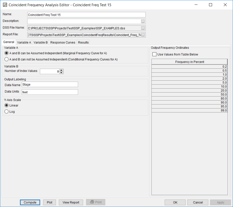
Shown in Figure 2 are the general settings for this coincident frequency analysis. For this analysis, the A and B can be Assumed Independent (Marginal Frequency Curve for A) option was selected. This choice would be determined by performing a correlation analysis between variables A and B; little correlation would indicate that variables A and B could be assumed independent. The number of variable B index values was set to 9, the Data Name was set to "Stage" and the Data Units to "feet", and the y-axis scale was set to Linear.
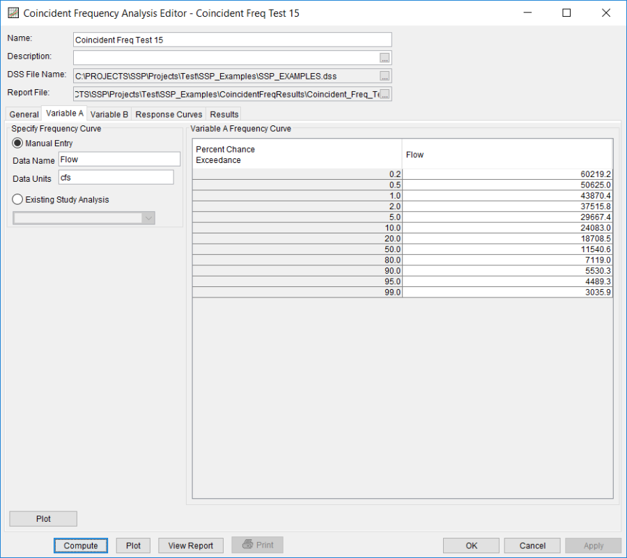
Shown in Figure 3 is the Coincident Frequency Analysis editor with the Variable A Tab selected. The Manual Entry option was selected and a Data Name of "Flow" and Data Units of "cfs" were entered. The frequency curve values were manually entered into the Variable A Frequency Curve table.
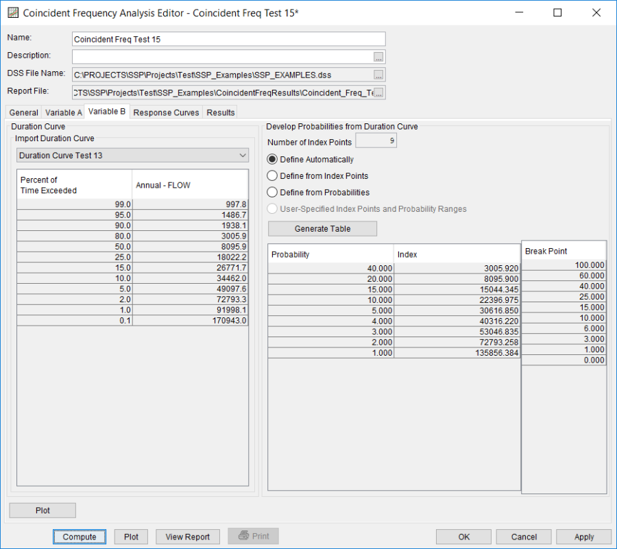
Shown in Figure 4 is the Coincident Frequency Analysis editor with the Variable B tab selected. The Duration Curve from Test 13 was selected in the drop-down list. Once selected, the duration curve table automatically fills with the computed ordinates from the duration curve. In the Develop Probabilities from Duration Curve panel, the Define Automatically option was selected. This option uses a predefined probability pattern to discretize the duration curve into index points. The Generate Table button was pressed in order activate the predefined probability pattern. In this example, the first index value is 3005.92 (cfs). This value is taken at the midpoint between percent of time exceeded values at 100 and 60 percent (from Duration Curve Test 13). This index value is assigned a probability of 40 percent; this flow value is used to represent 40% of the possible outcomes. The second index value is 8095.9. This value is taken at the midpoint between percent of time exceeded values at 60 and 40 percent and is assigned a probability of 20 percent.
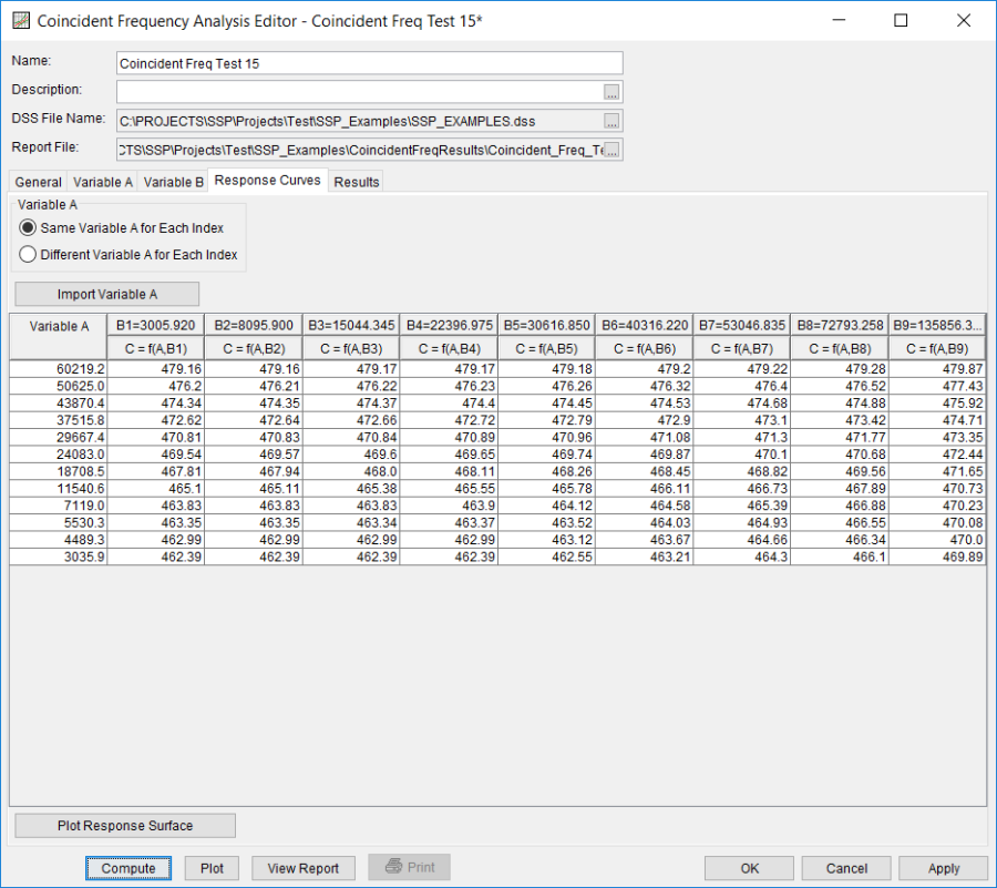
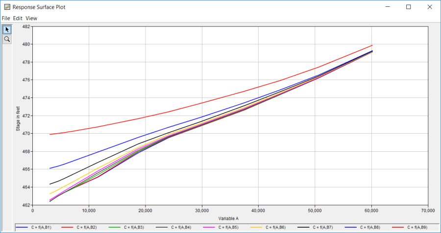
Once the Variable A and Variable B tabs have been completed, the user can populate the response curves table. Figure 5 shows the Response Curves tab for Coincident Freq Test 15. The Same Variable A for Each Index option was selected and the Import Variable A button was pressed to automatically copy values from the Variable A tab and fill in the Variable A column. The remaining columns in the table were populated with results from a hydraulics model. For example, the first value in the second column is 479.16. This value is the stage at the point of interest given a flow of 60219.18 (cfs) on the tributary (variable A) and a flow of 3005.92 (cfs) on the mainstem (variable B). A total of 108 simulations were required from the hydraulics model to fill in the response curves table. Figure 6 shows a plot of the response surface. The plot shows variable A (x-axis) and variable C (y-axis). For this example, the response surface shows that flows greater than 53000 (7th index point) on the mainstem affect the stage at the point of interest on the tributary. When the flow in the mainstem is below 53000 (cfs), only the flow on the tributary affects the stage at the point of interest.
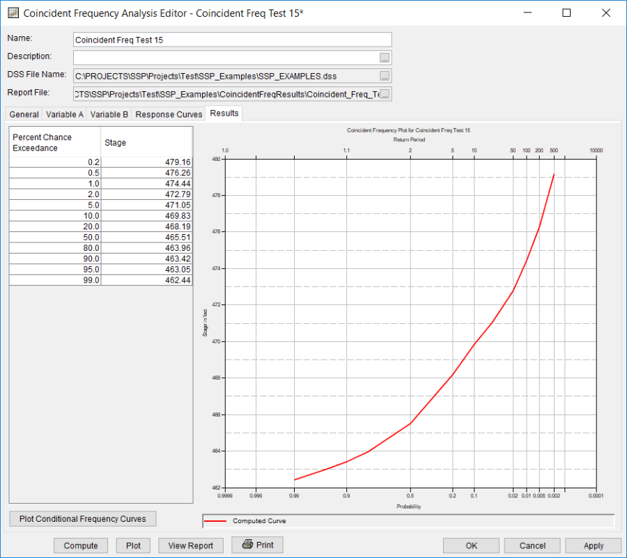
Press the Compute button to perform the analysis. Once the computations have been completed, a message window will open stating Compute Complete. Close this window and then select the Results tab. The results tab should resemble Figure 7. The left portion of the results tab contains the computed variable C frequency curve and the right portion of the results tab contains a plot of the computed variable C frequency curve.
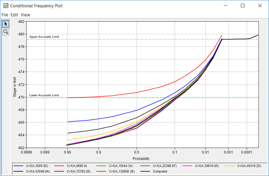
By pressing the Plot Condition Frequency Curves, the user can plot the response curves entered on the Response Curves tab along with the computed curve and the upper and lower accurate limits, as shown in Figure 8.
The tabular and graphical results can be sent to the printer or the windows clipboard for transfer into another piece of software. To print the tabular results, select Print from the bottom of the analysis window. To send the tabular results to the windows clipboard, highlight the data you want to send to the clipboard and then press the Control-C key sequence. To print the graphical results, first bring up the graphical plot by pressing the Plot button from the bottom of the analysis. Then select Print from the File menu. To send the graphic to the windows clipboard, select Copy to Clipboard from the File menu.
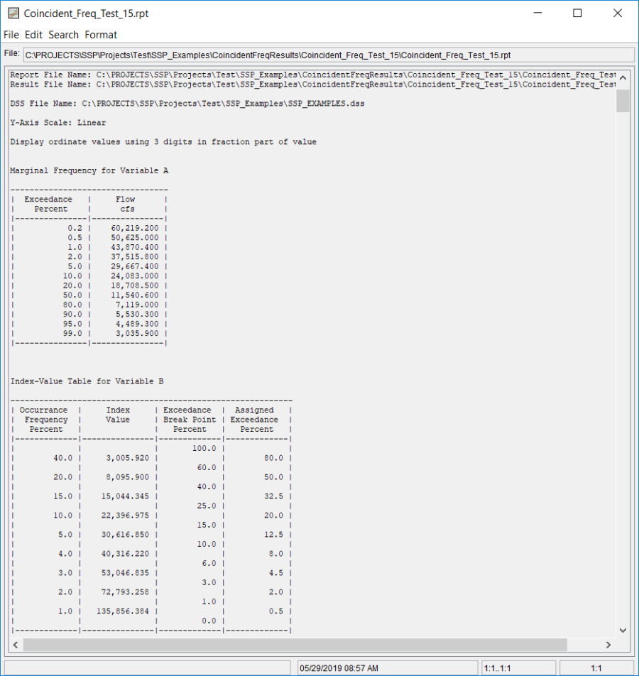
In addition to the tabular and graphical results, there is a report file that shows input data and results. To review the report file, press the View Report button at the bottom of the analysis window. When this button is selected a text viewer will open the report file and display it on the screen. Shown in Figure 9 is the report file for Coincident Freq Test 15.
