Download PDF
Download page Example 20. Distribution Fitting, Analyzing Model Uncertainty Using a Time Series of Annual Maximum Streamflow.
Example 20. Distribution Fitting, Analyzing Model Uncertainty Using a Time Series of Annual Maximum Streamflow
This example demonstrates how to use the Distribution Fitting analysis to analyze model uncertainty (i.e. choice of analytical distribution and fitting method) using a time series of annual maximum streamflow. The data for this example consists of an instantaneous peak annual maximum series of streamflow for a location along the Potomac River near Point of Rocks, MD. This stream gage is operated by the USGS (gage ID: 01638500). The period of record used for this example is from 1889 to 2016. To view the data from HEC-SSP, right-click on the data record labeled "Potomac River-Flow-Annual Peak" in the study explorer and then select Plot. A plot of the data will appear as shown in Figure 1.
A Distribution Fitting analysis has been developed for this example. A distribution | fitting method combination has not been selected within the SSP Examples study. To visualize, inspect, and select a distribution | fitting method combination, the following steps should be used. To open the Distribution Fitting analysis editor for this example, either double-click on the analysis labeled Distribution Fitting Test 20 from the study explorer, or from the Analysis menu, select open, then select Distribution Fitting Test 20 from the list of available analyses. When this analysis is opened, the Distribution Fitting editor will appear as shown in Figure 2.
For this analysis, the instantaneous peak streamflow data was used without modifications. Summary statistics of the data can be accessed by pressing the Data Summary Statistics button near the bottom of the Distribution Fitting editor while on the Data tab, as shown in Figure 3.
On the Analysis tab, several analytical distributions and fitting methods are available for selection. As shown in Figure 4, the Display All Distributions radio button was selected within the Distribution Filter panel to display all of the available analytical distributions while the default Product Moments fitting method was changed to L-Moments by clicking on the column header and selecting L-Moments. The Chi-Square goodness of fit test was selected by clicking on the column header and selecting Chi-Square. Additional output frequency ordinates were specified by clicking on the Plot Options button and adding them within the Output Frequency Ordinates panel, as shown in Figure 5. Several analytical distributions (some which poorly fit the data as well as some that fit the data well) were then selected and compared. CDF, PDF, PP, QQ, and CDF-Plotting Position plots comparing these distributions are shown in Figure 6, Figure 7, Figure 8, Figure 9, and Figure 10.


Kolmogorov-Smirnov and Chi-Square summary statistics can be accessed by pressing the Goodness of Fit Summary Statistics button near the top of the Distribution Fitting editor while on the Analysis tab, as shown in Figure 11. 
In this example, the Generalized Logistic Distribution fit using L-Moments was selected by clicking the Accept Selected Distribution button near the bottom of the Distribution Fitting editor while having that row selected on the Analysis tab. Upon clicking this button, confidence limits and an expected probability curve were automatically computed using the options specified within the Plot Options and Confidence Limits and Expected Probability Options editors. However, the default confidence limits and expected probability options were modified by clicking on the Plot Options and Confidence Limits and Expected Probability Options buttons near the bottom of the Distribution Fitting editor. Specifically, the Log option was selected within the Expected Probability Ordinates panel (which computes the expected probability curve using log base 10 values), the Z Alpha value was set to 99%, and the Maximum Iterations were set to 1,000,000, as shown in Figure 12. Upon clicking the OK button, updated confidence limits and an expected probability curve were recomputed. The accepted distribution | fitting method was used to populate the Results tab, as shown in Figure 13.

In addition to the tables and plot available on the Results tab, CDF, PDF, and CDF-Plotting Position plots of the data and accepted distribution | fitting method can be obtained by double left-clicking on the plot of interest. The CDF-Plotting Position plot of the data and accepted distribution | fitting method is shown in Figure 14.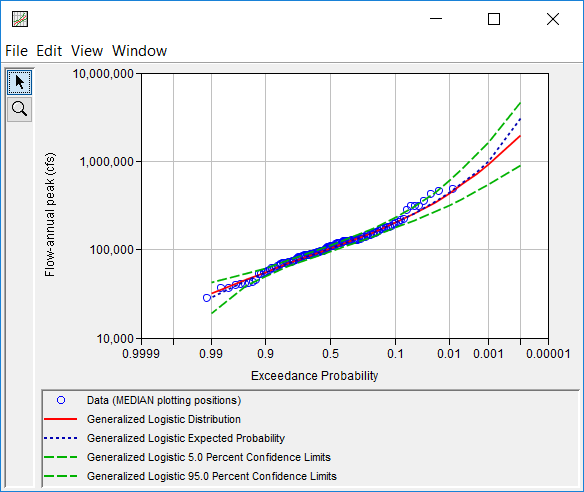
In addition to the tabular and graphical results, there is a report file that shows the input data, data filters that were applied, processed data, data summary statistics, all available analytical distributions for the selected fitting method and their corresponding parameters, selected goodness of fit summary scores for each analytical distribution, and the accepted distribution | fitting method. Different types and amounts of information will be contained within the report file depending upon the data and the options that have been selected for the analysis. To review the report file, press the View Report button at the bottom of the analysis window. When this button is selected a text viewer will open the report file and display it on the screen, as shown in Figure 15. 