Download PDF
Download page Example 10. Systematic and Historical Record with Regional Skew – Schuylkill River at Berne, PA.
Example 10. Systematic and Historical Record with Regional Skew – Schuylkill River at Berne, PA
Example 10 exhibits the use of a regional skew coefficient and MSE with systematic and historical data. The regional skew and MSE were estimated for this location in conjunction with several other large subbasins within the Delaware River watershed (Goldman & Konieczki, 2009). Examples of additional regional skew studies can be found through online searched, from the U.S. Army Corps of Engineers, and USGS, amongst others. Several regional skew studies have been compiled and made available at the following location: https://acwi.gov/hydrology/Frequency/b17c/supplementary-materials/reports.html. The data for this example comes from the USGS gage 01470500 Schuylkill River at Berne, PA. The period of record used for this example contains 70 peaks beginning in 1942 and ending in 2016. A single period of missing data exists within this record. Also, a historic flood event occurred outside the period of gaging record in April 1942. The annual maximum series is plotted in Figure 1 and tabulated in Table 1.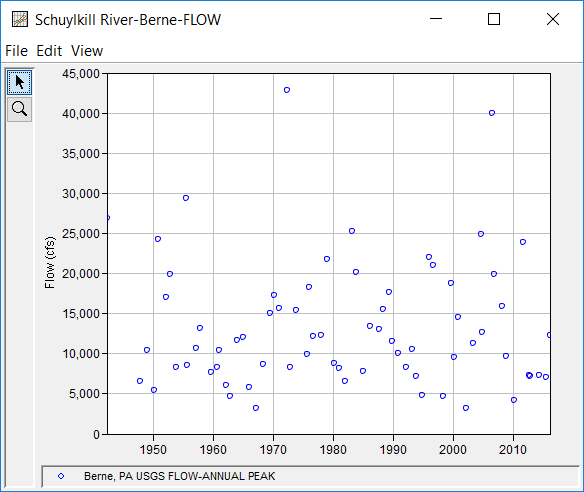
Table 1. Schuylkill River at Berne, PA Annual Peak Flow Record.
Date | Flow (cfs) |
|---|---|
30 Apr 1942 | 26900 |
08 Nov 1947 | 6500 |
30 Dec 1948 | 10400 |
23 Mar 1950 | 5430 |
04 Dec 1950 | 24200 |
11 Mar 1952 | 17000 |
22 Nov 1952 | 19900 |
07 Dec 1953 | 8290 |
19 Aug 1955 | 29400 |
15 Oct 1955 | 8580 |
06 Apr 1957 | 10700 |
21 Dec 1957 | 13100 |
03 Sep 1959 | 7710 |
20 Sep 1960 | 8290 |
26 Feb 1961 | 10400 |
12 Mar 1962 | 6010 |
10 Nov 1962 | 4720 |
25 Jan 1964 | 11700 |
08 Feb 1965 | 12000 |
14 Feb 1966 | 5850 |
06 Mar 1967 | 3220 |
31 May 1968 | 8640 |
02 Aug 1969 | 15000 |
02 Apr 1970 | 17300 |
13 Feb 1971 | 15600 |
22 Jun 1972 | 42800 |
08 Nov 1972 | 8290 |
21 Dec 1973 | 15400 |
26 Sep 1975 | 9920 |
26 Jan 1976 | 18300 |
09 Oct 1976 | 12100 |
26 Jan 1978 | 12300 |
25 Jan 1979 | 21700 |
21 Mar 1980 | 8780 |
11 Feb 1981 | 8110 |
03 Feb 1982 | 6600 |
16 Apr 1983 | 25300 |
14 Dec 1983 | 20100 |
12 Feb 1985 | 7850 |
15 Mar 1986 | 13400 |
13 Sep 1987 | 13000 |
19 May 1988 | 15500 |
06 May 1989 | 17600 |
16 Nov 1989 | 11500 |
04 Dec 1990 | 10000 |
27 Mar 1992 | 8280 |
11 Apr 1993 | 10500 |
05 Dec 1993 | 7210 |
28 Nov 1994 | 4820 |
19 Jan 1996 | 22000 |
19 Oct 1996 | 21000 |
12 May 1998 | 4720 |
16 Sep 1999 | 18700 |
22 Mar 2000 | 9530 |
17 Dec 2000 | 14500 |
15 Apr 2002 | 3230 |
21 Jun 2003 | 11300 |
18 Sep 2004 | 24900 |
28 Nov 2004 | 12700 |
28 Jun 2006 | 39900 |
17 Nov 2006 | 19900 |
05 Mar 2008 | 15900 |
12 Dec 2008 | 9720 |
14 Mar 2010 | 4210 |
08 Sep 2011 | 23900 |
18 Sep 2012 | 7240 |
21 Dec 2012 | 7220 |
16 May 2014 | 7240 |
01 Jul 2015 | 7040 |
25 Feb 2016 | 12300 |
A Bulletin 17 Analysis using EMA and Bulletin 17C procedures has been developed for this example. To open the analysis, either double-click on the analysis labeled "B17C Example 10" from the Study Explorer or from the Analysis menu select open, then select "B17C Example 10" from the list of available analyses. When "B17C Example 10" is selected, the Bulletin 17 analysis editor will appear as shown in Figure 2 As shown, the Skew option was set to use the Weighted Skew. To use the weighted skew option, the user must enter a value for the Regional Skew and the Regional MSE. In this example, a regional skew of 0.001 was used along with a Regional Skew MSE of 0.064.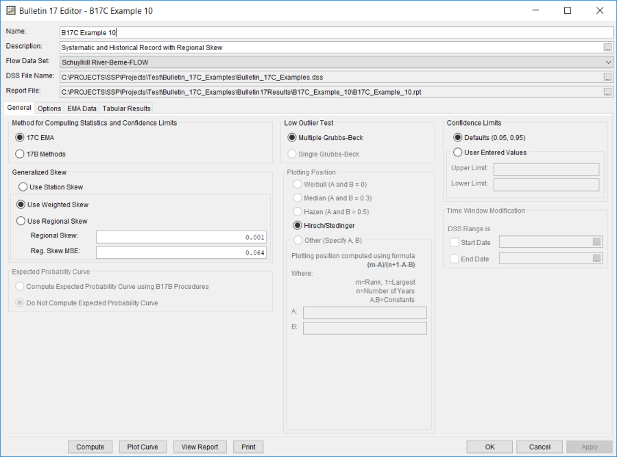
No changes to the Options tab are necessary. The EMA Data tab for this example is shown in Figure 3. This example uses an annual maximum series consisting of both systematic data and an historical event in April 1942. Also, the record is broken with a period of missing data spanning 1943 – 1947. Since 17C EMA requires a non zero – inf perception threshold for all periods of missing data, two perception thresholds are required. In this case, the peak discharge estimate associated with the April 1942 event can be used to inform the perception threshold for the period of missing annual peak flow data. The use of a perception threshold of 26000 – inf for this period of missing data implies that had a flood event occurred with a peak flow greater than 26,000 cfs, someone would have measured and recorded it. Since the April 1942 event was not directly measured, the perception threshold should span 1942 – 1947. Once the perception thresholds have been entered as shown in Figure 3, click the Apply Thresholds button to assign the complementary flow ranges for the periods of missing data. Finally, the April 1942 event should be set to the historical data type, as denoted by a USGS peak flow rate qualification code of "7".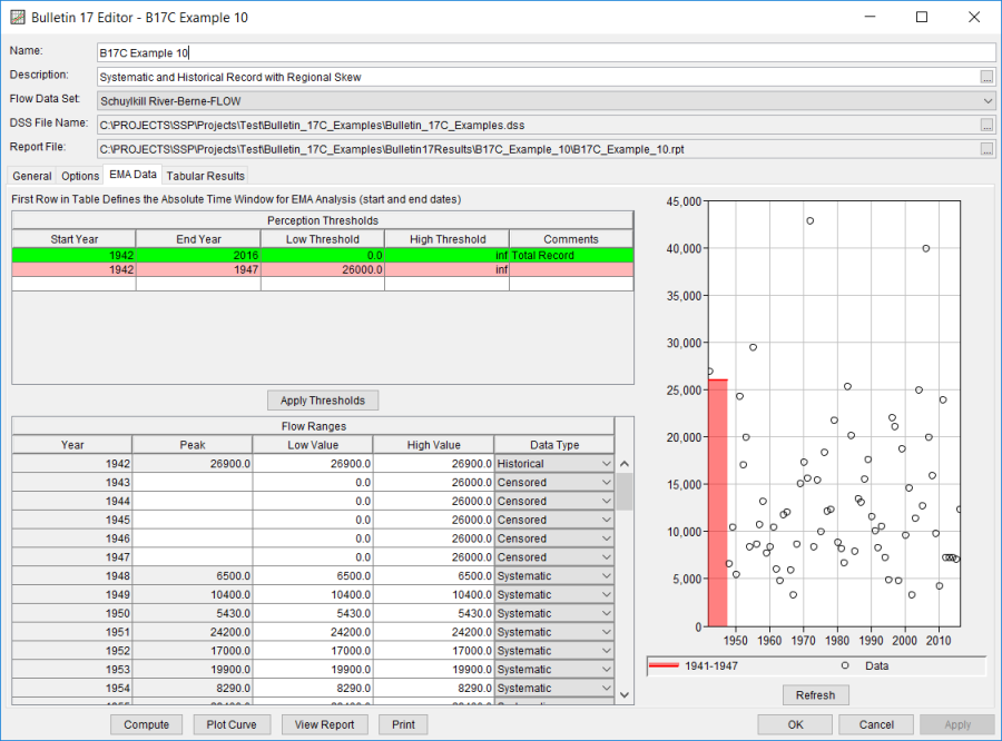
Once all of the General and EMA Data tab settings are set or selected, the user can press the Compute button to perform the analysis. Once the computations have been completed, a message window will open stating Compute Complete. Close this window and then select the Tabular Results tab. The analysis window should resemble Figure 4.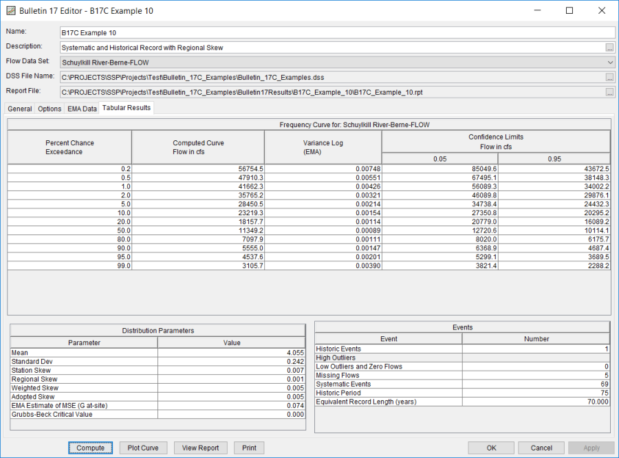
In addition to the tabular results, a graphical plot of the computed frequency curves can be obtained by pressing the Plot Curve button at the bottom of the analysis window. The Log Pearson Type III distribution fit using EMA to the input annual maximum flow data set, the 5% and 95% confidence limits, and the computed plotting positions are shown in Figure 5.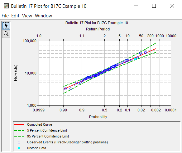
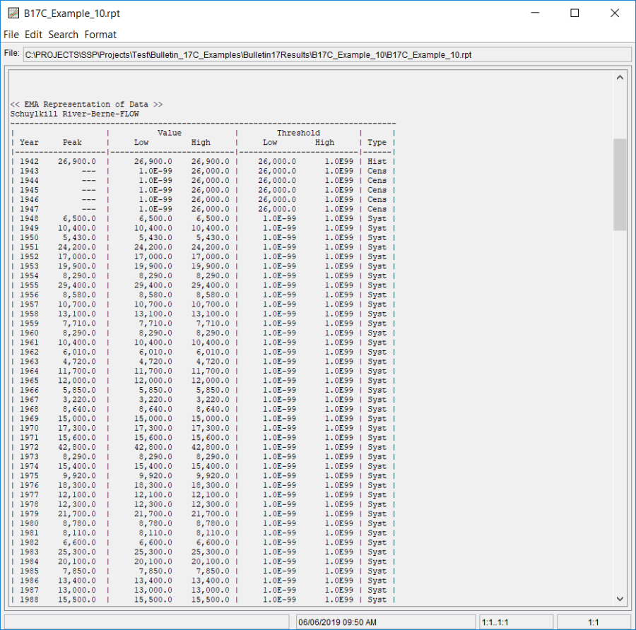
As shown in Figure 6, the 1942 – 1947 period used a perception threshold of 26000 – inf. Since the 1943 – 1947 period was missing, the complementary flow range of 0 – 26000 cfs was assigned and used within the computations.