Download PDF
Download page Expanding Window - Bushkill Creek.
Expanding Window - Bushkill Creek
In the SSP_Examples.ssp study, the Bulletin 17 analysis Bushkill_ExpandingWindow illustrates how to utilize the Expanding Window computational option. In this example, an initial period of 20 years is incrementally expanded by 5 years to explore how individual flood peaks impact a flow-frequency curve as well as the parameters of the Log Pearson Type III Distribution.
Input Data
The Bushkill Creek at Shoemakers, PA stream gage has an annual peak record consisting of 111 peaks beginning in 1909 and ending in 2019, as shown in Figure 1. The annual peak flow record is tabulated within Table 1.
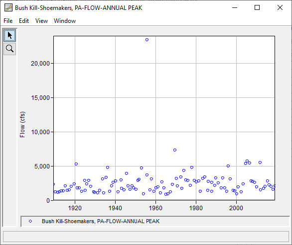
Table 1. Bushkill Creek at Shoemakers, PA Annual Peak Flow Record
| Date | Flow (cfs) |
|---|---|
| 20 Feb 1909 | 2270 |
| 07 Mar 1910 | 1190 |
| 14 Jun 1911 | 1120 |
| 15 Mar 1912 | 1190 |
| 28 Mar 1913 | 1350 |
| 29 Mar 1914 | 1350 |
| 24 Feb 1915 | 2070 |
| 02 Apr 1916 | 1430 |
| 27 Mar 1917 | 1510 |
| 26 Feb 1918 | 1970 |
| 22 Jul 1919 | 2380 |
| 24 Jul 1920 | 5250 |
| 10 Mar 1921 | 1780 |
| 08 Mar 1922 | 1780 |
| 24 Mar 1923 | 1270 |
| 30 Sep 1924 | 2830 |
| 12 Feb 1925 | 1430 |
| 16 Nov 1925 | 2380 |
| 16 Nov 1926 | 2830 |
| 19 Oct 1927 | 1970 |
| 15 Mar 1929 | 1190 |
| 18 Nov 1929 | 1150 |
| 29 Mar 1931 | 1080 |
| 01 Apr 1932 | 1430 |
| 16 Sep 1933 | 3070 |
| 12 Apr 1934 | 1040 |
| 10 Jul 1935 | 3330 |
| 18 Mar 1936 | 4770 |
| 06 Apr 1937 | 1240 |
| 25 Jan 1938 | 2070 |
| 06 Dec 1938 | 2540 |
| 31 Mar 1940 | 2790 |
| 06 Apr 1941 | 1220 |
| 28 Sep 1942 | 2920 |
| 30 Dec 1942 | 1710 |
| 25 Apr 1944 | 1500 |
| 19 Jul 1945 | 3900 |
| 28 May 1946 | 2080 |
| 06 Apr 1947 | 1580 |
| 21 Mar 1948 | 2080 |
| 31 Dec 1948 | 1780 |
| 29 Mar 1950 | 1540 |
| 31 Mar 1951 | 2860 |
| 08 Nov 1951 | 2980 |
| 11 Dec 1952 | 4680 |
| 07 Dec 1953 | 928 |
| 19 Aug 1955 | 23400 |
| 16 Oct 1955 | 3680 |
| 06 Apr 1957 | 1460 |
| 21 Dec 1957 | 3050 |
| 06 Mar 1959 | 1260 |
| 05 Apr 1960 | 1800 |
| 26 Feb 1961 | 1890 |
| 08 Apr 1962 | 1060 |
| 27 Mar 1963 | 2680 |
| 10 Mar 1964 | 1800 |
| 09 Feb 1965 | 804 |
| 06 Mar 1966 | 880 |
| 15 Mar 1967 | 1200 |
| 30 May 1968 | 2290 |
| 28 Jul 1969 | 7300 |
| 02 Apr 1970 | 3130 |
| 23 Oct 1970 | 2070 |
| 23 Jun 1972 | 3360 |
| 03 Feb 1973 | 1730 |
| 21 Dec 1973 | 4280 |
| 08 Dec 1974 | 2910 |
| 28 Jan 1976 | 2830 |
| 25 Feb 1977 | 2120 |
| 09 Jan 1978 | 4720 |
| 25 Jan 1979 | 2830 |
| 22 Mar 1980 | 2670 |
| 12 May 1981 | 2770 |
| 04 Feb 1982 | 1300 |
| 16 Apr 1983 | 3160 |
| 05 Apr 1984 | 3340 |
| 27 Sep 1985 | 1420 |
| 15 Mar 1986 | 2730 |
| 13 Sep 1987 | 2580 |
| 30 Nov 1987 | 1260 |
| 06 May 1989 | 2120 |
| 20 Oct 1989 | 3260 |
| 04 Dec 1990 | 2470 |
| 31 May 1992 | 1780 |
| 01 Apr 1993 | 3210 |
| 28 Mar 1994 | 1750 |
| 08 Mar 1995 | 1280 |
| 27 Jan 1996 | 4990 |
| 02 Dec 1996 | 3060 |
| 12 May 1998 | 1450 |
| 24 Jan 1999 | 1360 |
| 28 Feb 2000 | 895 |
| 17 Dec 2000 | 1930 |
| 29 May 2002 | 1210 |
| 22 Jun 2003 | 2340 |
| 18 Sep 2004 | 5330 |
| 03 Apr 2005 | 5670 |
| 28 Jun 2006 | 5380 |
| 16 Apr 2007 | 2790 |
| 09 Mar 2008 | 2750 |
| 12 Dec 2008 | 2590 |
| 25 Jan 2010 | 1940 |
| 28 Aug 2011 | 5480 |
| 08 Dec 2011 | 1480 |
| 11 Jun 2013 | 1740 |
| 01 May 2014 | 2030 |
| 01 Jul 2015 | 2790 |
| 25 Feb 2016 | 2220 |
| 07 Apr 2017 | 1970 |
| 25 Feb 2018 | 1550 |
| 24 Jan 2019 | 2070 |
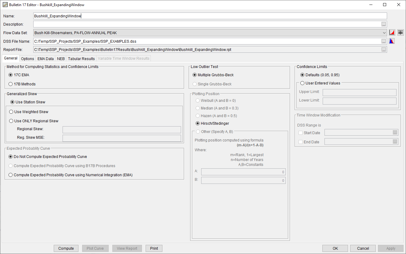
A Bulletin 17 Analysis using Bulletin 17C procedures and the Variable Time Window | Expanding Window compute option has been developed for this example. To open the analysis, either double-click on the analysis labeled Bushkill_ExpandingWindow from the Study Explorer or from the Analysis menu select open, then select Bushkill_ExpandingWindow from the list of available analyses. When Bushkill_ExpandingWindow is selected, the Bulletin 17 analysis editor General tab will appear as shown in Figure 2. As shown, the 17C EMA computational option was selected along with all the subsequent default options.
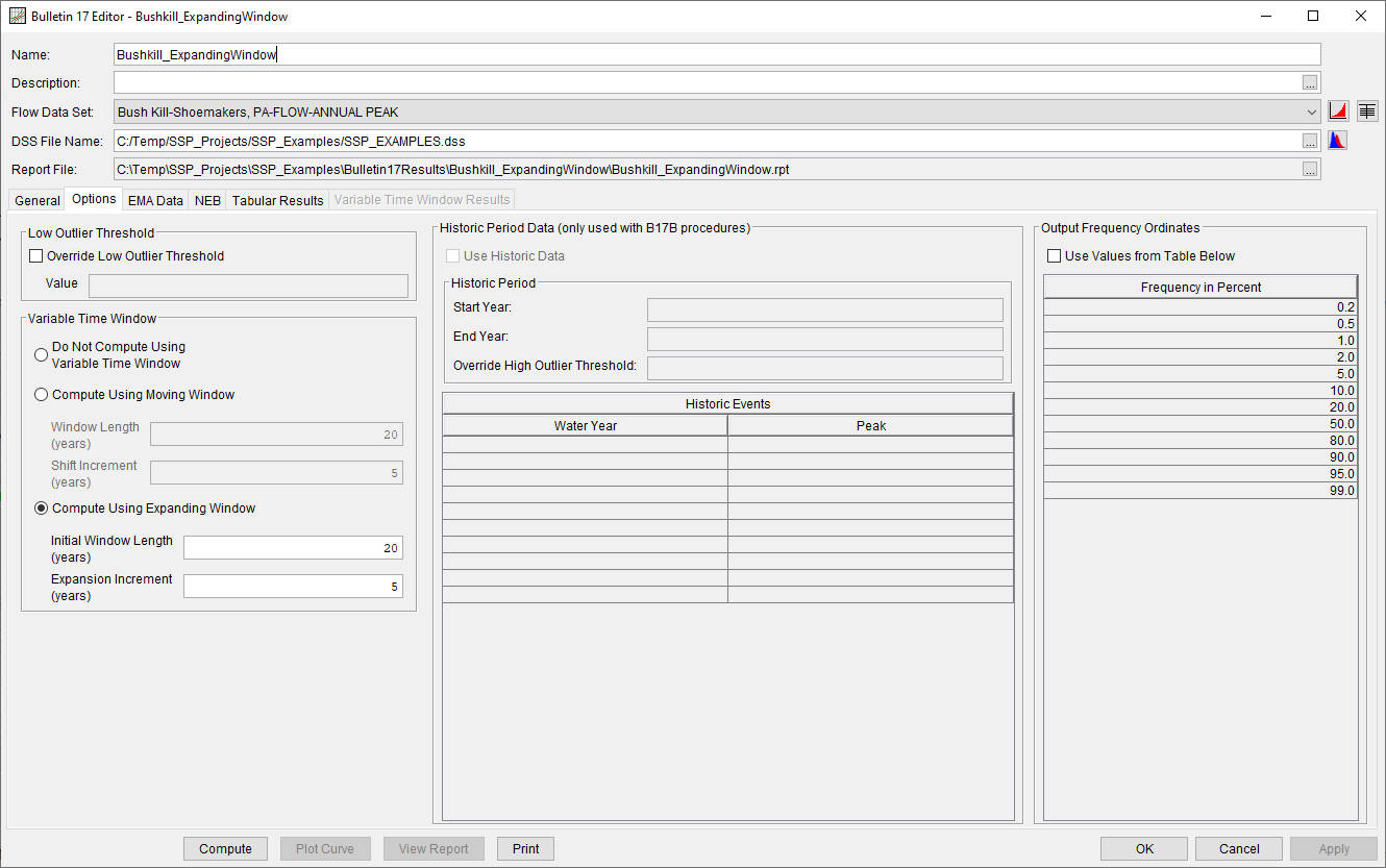
On the Options tab, the Compute Using Expanding Window option was selected within the Variable Time Window panel. An Initial Window Length of 20 years and an Expansion Increment of 5 years was entered, as shown in Figure 3.
The EMA Data tab for this example is shown in Figure 4. Since this example uses an annual maximum series consisting entirely of systematic data with a complete record, a single zero – inf perception threshold is adequate. No modifications to the default flow ranges and data types are necessary.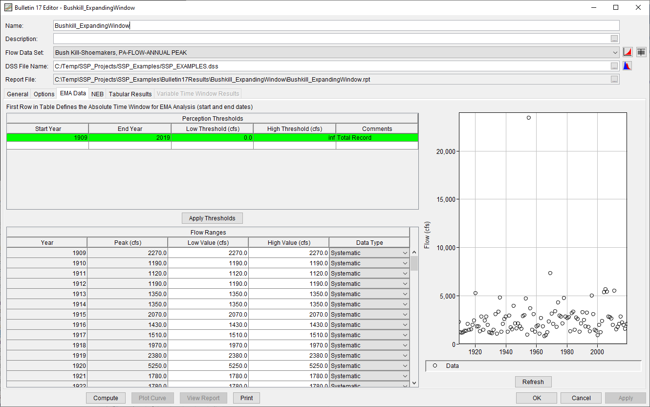
Computing the Analysis
Once all of the General, Options, and EMA Data tab settings are set or selected, the user can press the Compute button to perform the analysis. A Compute Warnings message will be shown noting that the final expansion increment was less than 5 years. Once the computations have been completed, a message window will open stating Compute Complete.
Close these windows and then select the Tabular Results tab. The analysis window should resemble Figure 5.
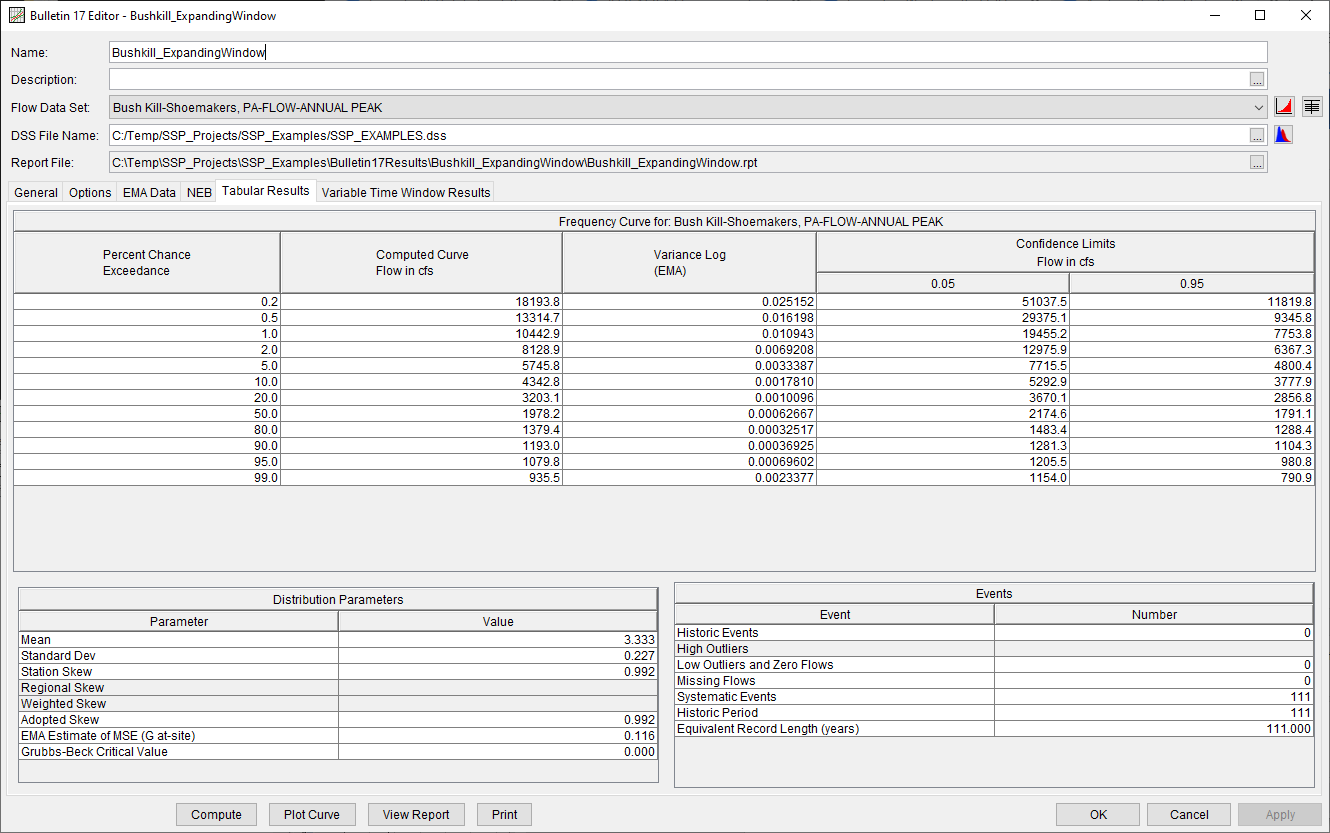
When using the Expanding Time Window compute option, the Tabular Results tab will only contain the results from the final time window computation. In this example, the final time window spans water years 1909 - 2019, which is 111 total years.
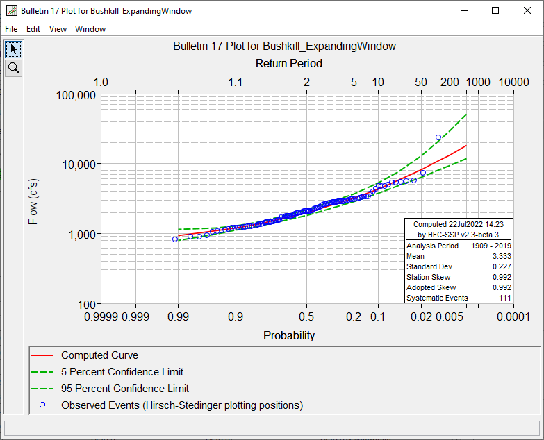
In addition to the tabular results, a graphical plot of the computed frequency curves for the final time window can be obtained by pressing the Plot Curve button at the bottom of the analysis window.
Expanding Time Window Results
Upon clicking the Variable Time Window Results tab, two sub-tabs become available: Flow and Statistics. The Flow sub-tab contains the evolution of quantile information for each time window and each of the frequency ordinates specified within the Options tab | Output Frequency Ordinates table, as shown within Figure 6.
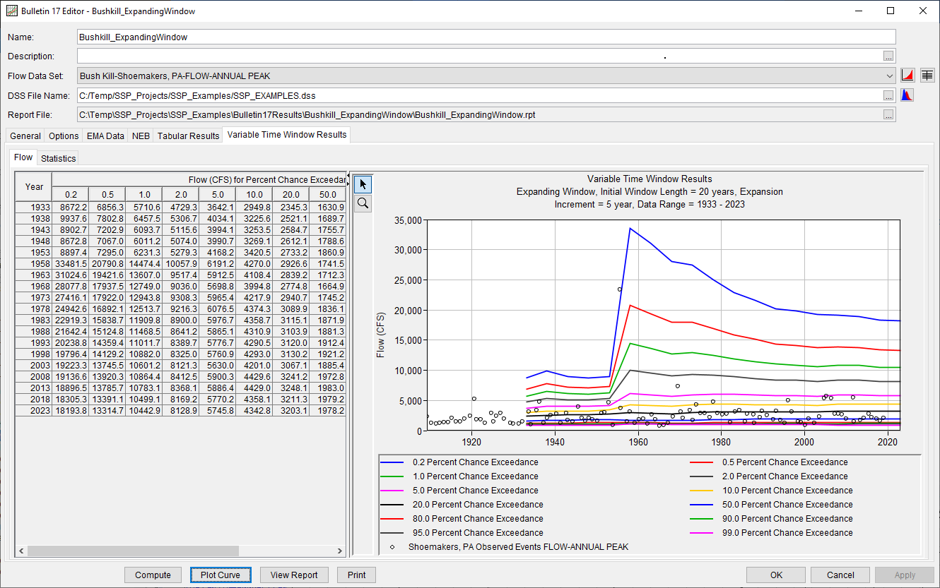
Within this example, 19 time windows were derived from the input data, as shown in Table 2.
Table 2. Time Windows for Bushkill_ExpandingWindow Bulletin 17 Analysis
| Begin Year | End Year | Number of Years |
|---|---|---|
| 1909 | 1933 | 25 |
| 1909 | 1938 | 30 |
| 1909 | 1943 | 35 |
| 1909 | 1948 | 40 |
| 1909 | 1953 | 45 |
| 1909 | 1958 | 50 |
| 1909 | 1963 | 55 |
| 1909 | 1968 | 60 |
| 1909 | 1973 | 65 |
| 1909 | 1978 | 70 |
| 1909 | 1983 | 75 |
| 1909 | 1988 | 80 |
| 1909 | 1993 | 85 |
| 1909 | 1998 | 90 |
| 1909 | 2003 | 95 |
| 1909 | 2008 | 100 |
| 1909 | 2013 | 105 |
| 1909 | 2018 | 110 |
| 1909 | 2019 | 111 |
The Statistics sub-tab contains the evolution of Log Pearson Type III parameters for each time window, as shown within Figure 7.
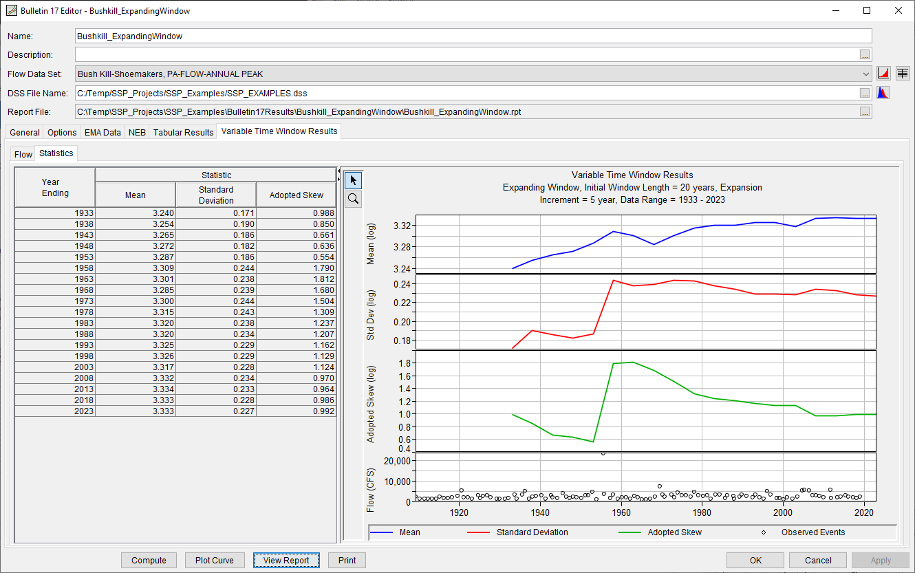
Notice the extreme event in 1955. The peak flow rate for the 1955 event was 23,400 cfs; whereas, the next largest flood was 7,300 cfs in 1969. The inclusion (or exclusion) of this flood event causes dramatic changes to the computed quantiles (e.g. 1/100 annual exceedance probability flow rate) as well LPIII parameters (e.g. skew).
Report File
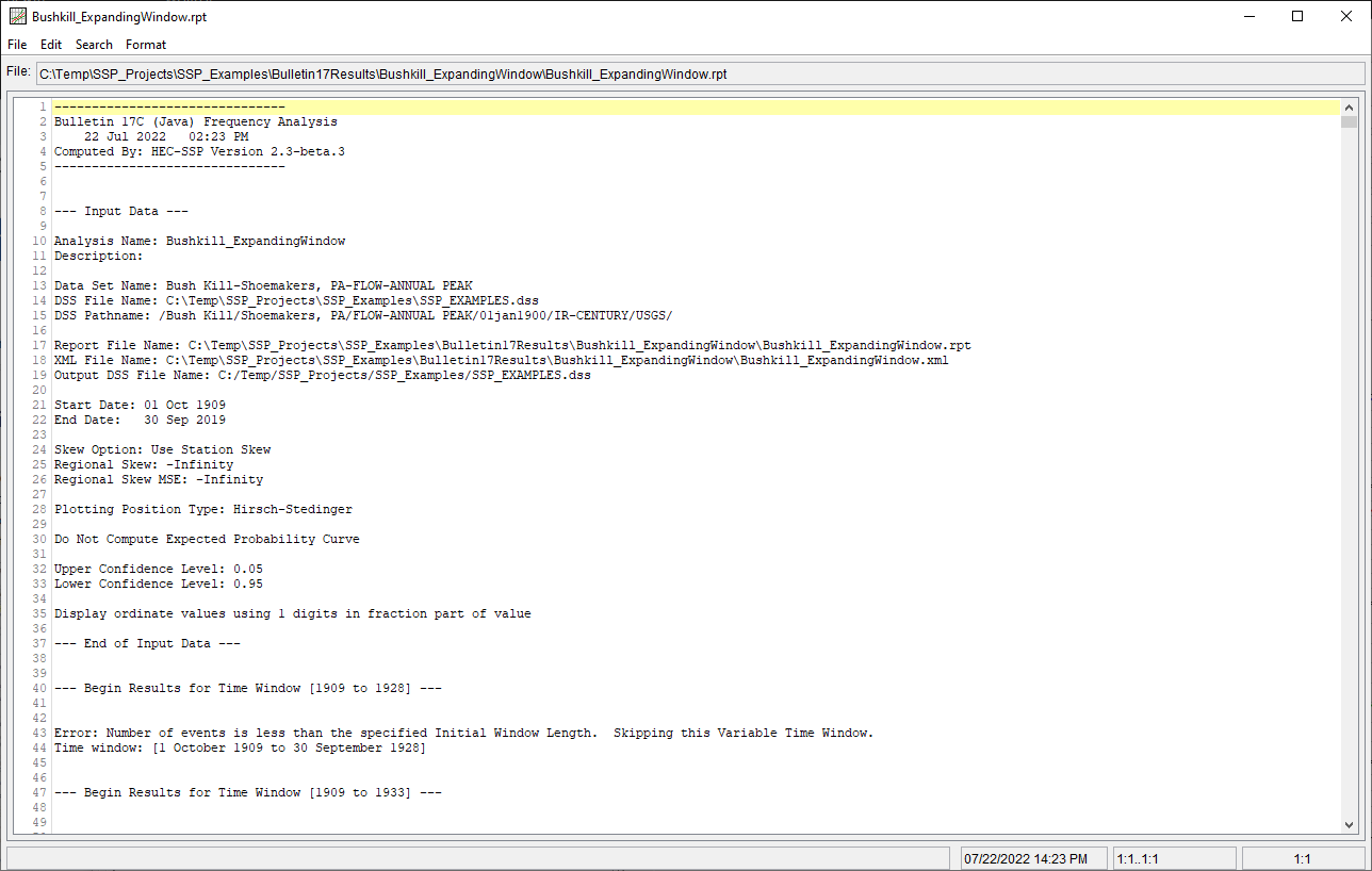
In addition to the tabular and graphical results, there is a report file that shows the order in which the calculations were performed. To review the report file, press the View Report button at the bottom of the analysis window. When this button is selected, a text viewer will open the file and display it on the screen. Shown in Figure 8 is the report file. The report file contains a listing of the input data, preliminary results, outlier and historical data tests, additional calculations needed, and the final frequency curve results for each of the time windows. Additionally, a final summarization of all the time windows is included. Different types and amounts of information will show up in the report file depending on the data and the options that have been selected for the analysis. The user should review the report file to understand how the Bulletin 17C procedures were applied for each time window.
