Download PDF
Download page Example 5. Confidence Limits and Low Threshold Discharge.
Example 5. Confidence Limits and Low Threshold Discharge
In the SSP_Examples.ssp study, the FFA Test 5 Bulletin 17 example analysis illustrates the use of user-entered confidence limits. Probabilities of 0.01 and 0.99 were entered for the computed confidence limit curves. This data set also includes two very low values, the higher of which is just above the default low outlier threshold. Therefore, this example also demonstrates the use of a user-entered low outlier threshold set to be higher than both values.
This example uses Bulletin 17B procedures (Interagency Advisory Committee on Water Data, 1982). Current Federal flood frequency guidance directs analysts to use Bulletin 17C procedures (England, et al., 2019). Bulletin 17C examples can be found here.
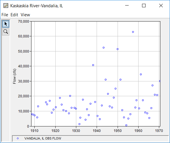
The data used for the FFA Test 5 example is from Kaskaskia River in Vandalia, Illinois. The period of record used for this example is from 1908 to 1970. To view the data in HEC-SSP, under the Data folder in the Study Pane, right-click on the data record labeled "Kaskaskia River-Vandalia, IL" and select Tabulate. The data will appear as shown in Figure 1.

To plot the data for this example, right-click on the data record and then select Plot. A plot of the data will appear as shown in Figure 2.
A Bulletin 17 and General Frequency analysis have been developed for this example; however, this example only displays the results of the Bulletin 17 analysis. To open the Bulletin 17 Editor for FFA Test 5, from the Study Pane under the Bulletin 17 Analysis folder, double-click on the FFA Test 5 analysis. Alternatively, from the Analysis menu select Open and then select FFA Test 5 from the list of available analyses in the Open Analysis dialog box. When FFA Test 5 is opened, the Bulletin 17 Editor - FFA Test 5 will appear as shown in Figure 3.

Shown in Figure 3 are the settings entered in the General tab that were used to perform this frequency analysis. As shown, the Generalized Skew option was set to use the Weighted Skew. To use the weighted skew option, the user must enter a value for the Regional Skew and the Regional Skew MSE. This selection requires the user to either look up a value from the generalized skew map of the United States, which is provided with Bulletin 17B, or develop a value from a regional analysis of nearby gages. In this example a value of -0.4 was taken from the generalized skew map of the U.S. from Bulletin 17B. Bulletin 17B suggests using a Regional Skew MSE of 0.302 whenever regional skew values are taken from the map.
The recommended procedure for estimating regional skew in Bulletin 17C is the Bayesian generalized least squares (B-GLS) method. Regional skew studies are available for many states through the Advisory Committee on Water Information, Subcommittee on Hydrology, Hydrologic Frequency Analysis Working Group website. Regional skew values presented in these reports supersede the values from the Bulletin 17B generalized skew map.
Also for the FFA Test 5 example, the Expected Probability Curve option was selected to be computed in addition to the Log Pearson III computed curve. The default method of Median plotting positions was selected. The default values for Confidence Limits were changed to 0.01 and 0.99.
Shown in Figure 4 is the Bulletin 17 Editor with the Options tab selected. As shown in Figure 4, a Low Outlier Threshold of 2000 cfs was entered. In the initial computation with this data (which the reader can reproduce by Computing without the "Use Low Outlier Threshold" box checked), the default low outlier threshold was 1,253 cfs, just below the second lowest value of 1,270 cfs. A look at the statistics and computed frequency curve from that run shows that the 1,270 cfs value is well below the computed curve and with a station skew of -0.21 the frequency curve does not fit the upper data well. By choosing to also censor the 1,270 cfs value with a threshold of 2000 cfs, the fit is improved. None of the other available options, such as Historic Period Data and the option to override the default Frequency Ordinates were selected for this test example.

Once all of the General and Optional settings are set or selected, the user can press the Compute button to perform the analysis. Once the computations have been completed a message window will open stating Compute Complete. Close this window and then select the Tabular Results tab from the analysis window. The analysis window should resemble Figure 5.

As shown in Figure 5, the Frequency Curve table contains the following results:
- Percent Chance Exceedance
- Computed Curve
- Expected Probability Curve
- Confidence Limits
On the bottom left-hand side of the Tabular Results tab is the Distribution Parameters table of Statistics for the observed station data (mean, standard deviation, station skew) and regional adjustment (regional skew, weighted skew, and adopted skew). Also on the bottom right-hand side of the Tabular Results tab is the number of Events table showing the number of historic events used in the analysis, number of high outliers found, number of low outliers, number of zero or missing data years, number of systematic events in the gage record, and the historic record length (only if historic data was entered). With the user-defined low-outlier threshold of 2000 cfs, there are two low-outliers detected. The analysis report shows the program omitted these values and used the Conditional Probability Adjustment to recompute the resulting frequency curve and statistics. The report file (described below) includes the preliminary computation before removal of outliers and the default and user-defined outlier thresholds, as well as the final frequency curve and statistics.
In addition to the tabular results, a graphical plot of the computed frequency curves can be obtained by pressing the Plot Curve button at the bottom of the analysis window. A plot of the results for this example is shown in Figure 6.

In addition to the tabular and graphical results, there is a report file that shows the order in which the calculations were performed. To review the report file, press the View Report button at the bottom of the Bulletin 17 Editor (Figure 5). The View Report button opens a text viewer window displaying the report file (e.g., FFA_Test_5.rpt). Shown in Figure 7 is the report file for FFA Test 5. The report file contains a listing of the input data, preliminary results, outlier and historical data tests, additional calculations needed, and the final frequency curve results. Different types and amounts of information will show up in the report file depending on the data and the options that have been selected for the analysis.
