Example 1. Systematic Record – Moose River at Victory, VT

Example 1 illustrates the computation of a peak flow frequency curve using EMA and Bulletin 17C procedures with an annual maximum series comprised of systematic flood peaks. For this example, USGS gage 01134500 Moose River at Victory, Vermont is used. The Moose River is located in the northeastern part of the state and flows mostly from north to south through very hilly terrain. The Moose River basin is approximately 75 square miles of nearly all forest (England, et al., 2018). Historically, it was an important logging area and some logging still continues today. Attempts at farming in the basin have generally failed due to the presence of shallow rocky soil. There are a small number of villages in the basin, but overall it is sparsely populated with only a few miles of paved roadway. There is also a large bog approximately a third of a mile upstream from the gage. The bog is part of the 5,000 acre Victory Basin Wildlife management area. While there is no streamflow regulation in the basin, the bog attenuates peaks in the basin. The Moose River at Victory, VT stream gage has an annual peak record consisting of 68 peaks beginning in 1947 and ending in 2014, as shown in Figure 1. The annual peak flow record is tabulated within Table 1.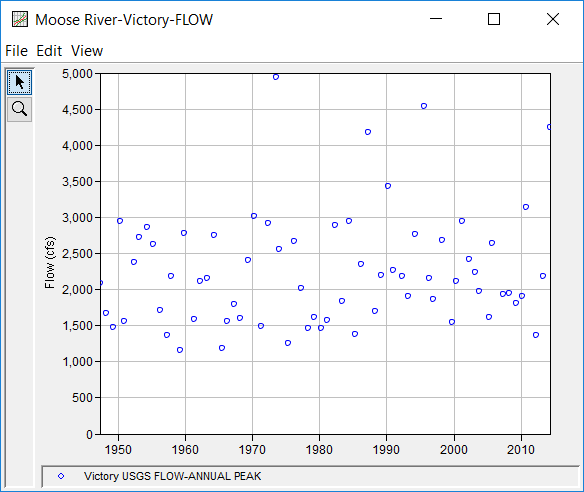


Table 1. Moose River at Victory, VT Annual Peak Flow Record.

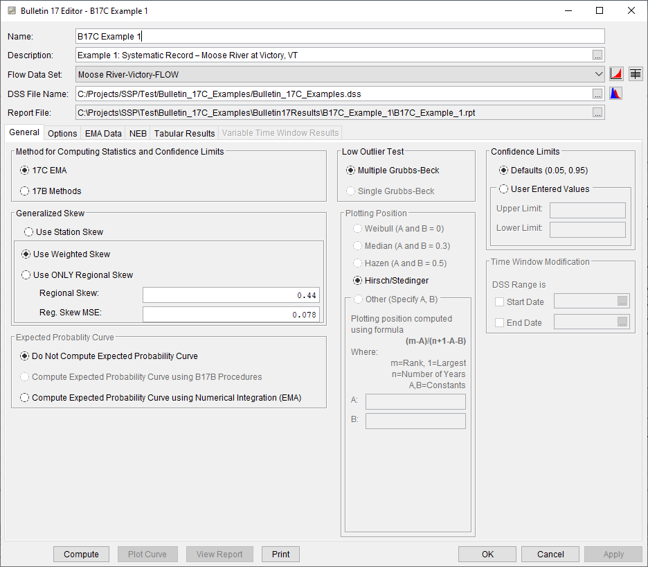
A Bulletin 17 Analysis using EMA and Bulletin 17C procedures has been developed for this example. To open the analysis, either double-click on the analysis labeled "B17C Example 1" from the Study Explorer or from the Analysis menu select open, then select "B17C Example 1" from the list of available analyses. When "B17C Example 1" is selected, the Bulletin 17 analysis editor will appear as shown in Figure 2. As shown, the Skew option was set to use the Weighted Skew. To use the weighted skew option, the user must enter a value for the Regional Skew and the Regional Skew MSE. In this example, a regional skew coefficient of 0.44 was used along with a Regional Skew MSE of 0.078.

The recommended procedure for estimating regional skew in Bulletin 17C is the Bayesian generalized least squares (B-GLS) method. Regional skew studies are available for many states through the Advisory Committee on Water Information, Subcommittee on Hydrology, Hydrologic Frequency Analysis Working Group website. Regional skew values presented in these reports supersede the values from the Bulletin 17B generalized skew map.

 

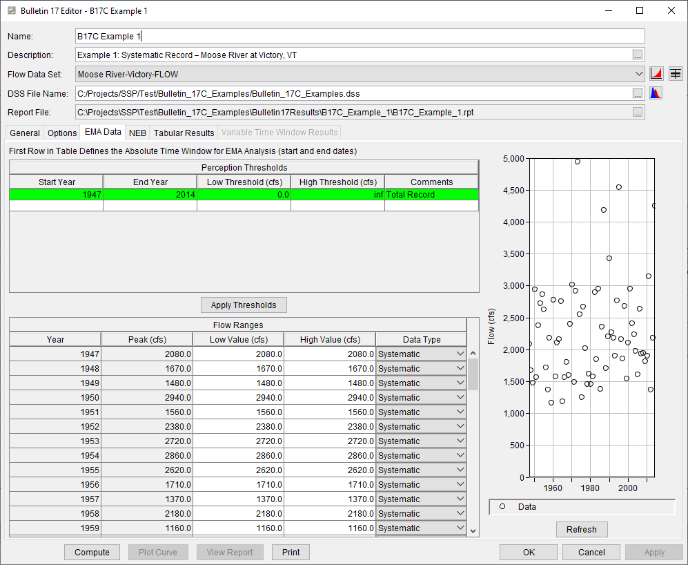
No changes to the Options tab are necessary. The EMA Data tab for this example is shown in Figure 3. Since this example uses an annual maximum series consisting entirely of systematic data with a complete record, a single zero – inf perception threshold is adequate. No modifications to the default flow ranges and data types are necessary.

Once all of the General and EMA Data tab settings are set or selected, the user can press the Compute button to perform the analysis. Once the computations have been completed, a message window will open stating Compute Complete. Close this window and then select the Tabular Results tab. The analysis window should resemble Figure 4. As shown in Figure 4, the Frequency Curve table contains the following results:

• Percent Chance Exceedance
• Computed Curve (Log Pearson Type III results)
• Confidence Limits (5% and 95% chance exceedance)

On the bottom left side of the results tab is a table of Distribution Parameters for the observed station data (mean, standard deviation, and station skew) and regional adjustment (regional skew, weighted skew, and adopted skew). Additionally, the computed EMA Estimate of MSE (G at-site) and Grubbs-Beck Critical Value are shown within this table. On the bottom right side of the results tab is an Events table showing the number of historic events used in the analysis, number of high outliers found, number of low outliers and zero flows found, number of missing flows, number of systematic events, the historic period in years, and the Equivalent Record Length in year.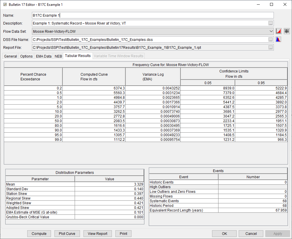

In addition to the tabular results, a graphical plot of the computed frequency curves can be obtained by pressing the Plot Curve button at the bottom of the analysis window. The Log Pearson Type III distribution fit using EMA and Bulletin 17C procedures to the input annual maximum flow data set, the 5% and 95% confidence limits, and the computed Hirsch/Stedinger plotting positions are shown in Figure 5.

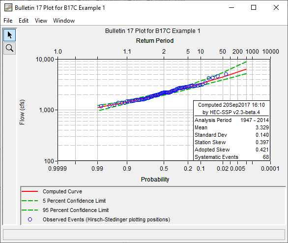
Because the annual peak flow record contains only systematic peaks with no historic information, no censored peaks, and no low outliers identified using the Multiple Grubbs-Beck Test, the fitted peak flow frequency curve using EMA and Bulletin 17C procedures is the same as that obtained using Bulletin 17B procedures. However, due to the appropriate consideration of the uncertainty in the skew coefficient within the Bulletin 17C procedures, the 5% and 95% confidence limits are different when compared against results obtained using Bulletin 17B procedures.

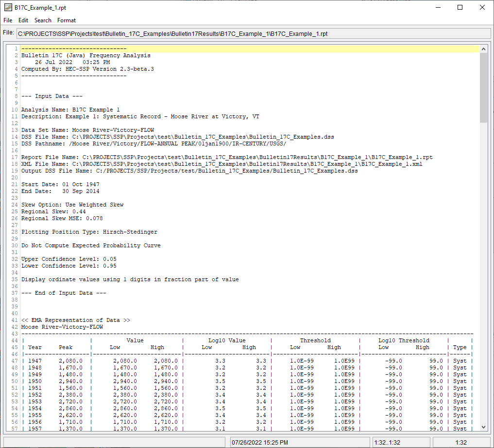
In addition to the tabular and graphical results, there is a report file that shows the order in which the calculations were performed. To review the report file, press the View Report button at the bottom of the analysis window. When this button is selected, a text viewer will open the file and display it on the screen. Shown in Figure 6 is the report file. The report file contains a listing of the input data, preliminary results, outlier and historical data tests, additional calculations needed, and the final frequency curve results. Different types and amounts of information will show up in the report file depending on the data and the options that have been selected for the analysis. The user should review the report file to understand how the Bulletin 17C procedures were applied.