Example 3. Broken Record – Back Creek near Jones Springs, WV

Example 3 illustrates the computation of a peak flow frequency curve using EMA and Bulletin 17C procedures with an annual maximum series comprised of a broken record of systematic flood peaks. For this example, USGS gage 01614000 Back Creek near Jones Springs, West Virginia is used. Back Creek is a tributary to the Potomac River; the 235 square mile watershed lies within the Valley and Ridge province in West Virginia (England, et al., 2018). Gage 01614000 has an annual peak record consisting of 56 peaks beginning in 1929 and ending in 2012. There are three "broken record" periods where the gage was discontinued: 1932-1937, 1976-1991, and 1999-2003. Thus, there are 28 years of missing data at this gage during the period 1929-2012. There is a historic flood that occurred on March 17, 1936, during one of the periods when the gage was discontinued. This flood is noted in the USGS Annual Water Data Report for this gage, available in the peak-flow file, and there is historical information available for this large flood (Grover, 1937).

The Back Creek near Jones Springs, WV stream gage has an annual peak record consisting of 56 annual peaks. Of the 56 annual peaks, the October 1942 flood slightly exceeds the March 1936 historic flood peak. Based on the historical flood information in Grover (1937) for the 1936 flood, and the large regional floods and historical floods described by Wiley and Atkins (2010) in West Virginia for the period 1888-1996, information from the March 1936 flood can be used as a perception threshold to represent the 28 years of missing information. This assumes that if a flood equal to or larger than the March 1936 event occurred when the gage was not operational, it would have been noted and recorded in some way. The annual maximum series is plotted in Figure 1 and tabulated in Table 1.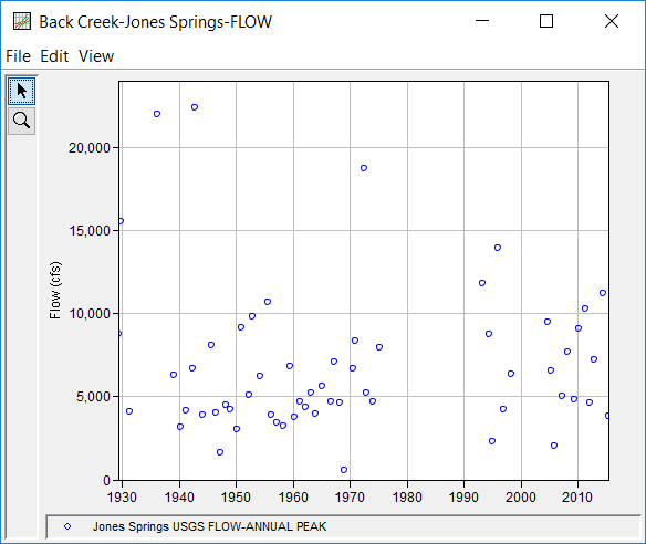


Table 1.  Back Creek near Jones Springs, WV Annual Peak Flow Record.

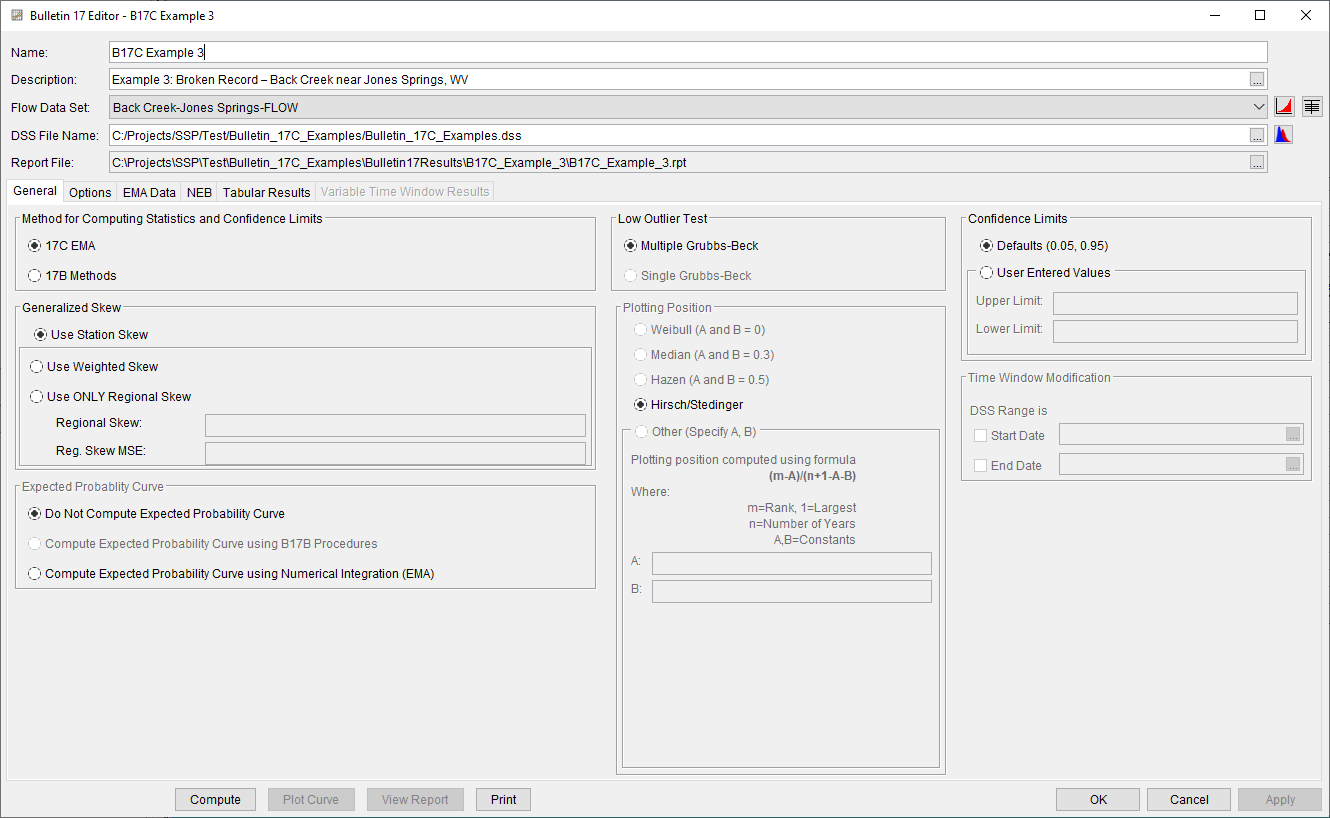
A Bulletin 17 Analysis using EMA and Bulletin 17C procedures has been developed for this example. To open the analysis, either double-click on the analysis labeled "B17C Example 3" from the Study Explorer or from the Analysis menu select open, then select "B17C Example 3" from the list of available analyses. When "B17C Example 3" is selected, the Bulletin 17 analysis editor will appear as shown in Figure 2. As shown, the Skew option was set to use the Station Skew.

No changes to the Options tab are necessary. The EMA Data tab for this example is shown in Figure 3. This example uses an annual maximum series consisting of both systematic data along with an historical event in March 1936. Also, the record is broken with multiple periods of missing with a complete record. Since 17C EMA requires a non zero – inf perception threshold for all periods of missing data, a total of four perception thresholds are required. In this case, the March 1936 event can be used to inform the perception thresholds for the periods of missing annual peak flow data. The use of a perception threshold of 21000 – inf for these periods of missing data implies that had a flood event occurred with a peak flow greater than 21,000 cfs, someone would have measured and recorded it. Once all four perception thresholds have been entered as shown in Figure 3, click the Apply Thresholds button to assign the complementary flow ranges for the periods of missing data. Finally, the March 1936 event should be set to the historical data type, as denoted by a USGS peak flow rate qualification code of "7", because it occurred during a period when the gage was discontinued.

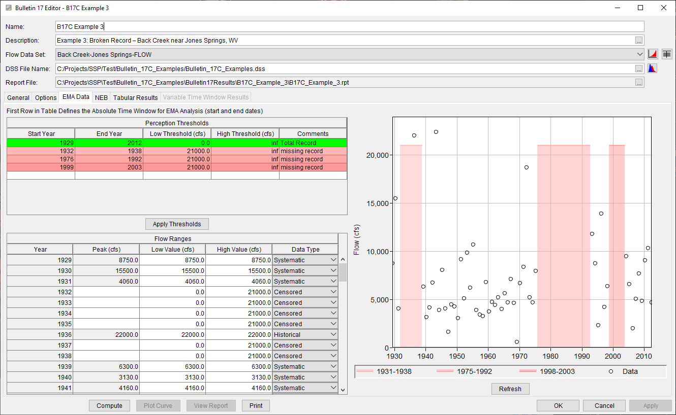
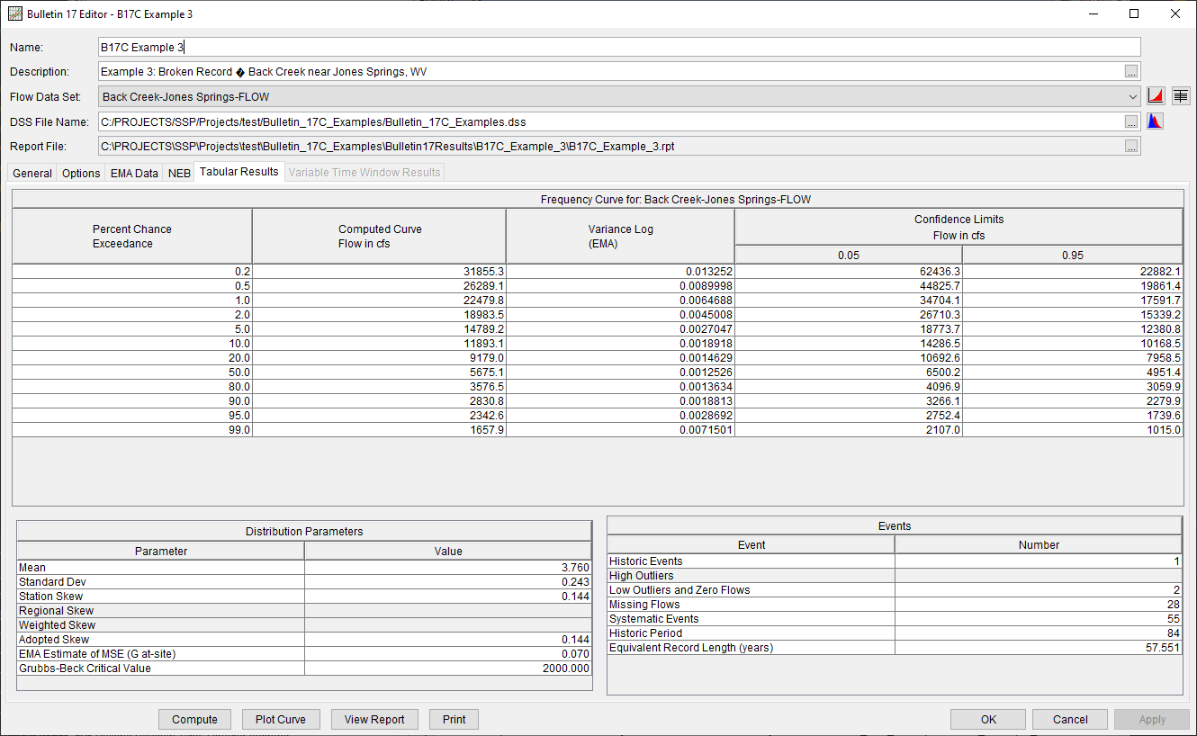
Once all of the General and EMA Data tab settings are set or selected, the user can press the Compute button to perform the analysis. Once the computations have been completed, a message window will open stating Compute Complete. Close this window and then select the Tabular Results tab. The analysis window should resemble Figure 4.

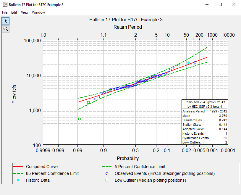
In addition to the tabular results, a graphical plot of the computed frequency curves can be obtained by pressing the Plot Curve button at the bottom of the analysis window. The Log Pearson Type III distribution fit using EMA to the input annual maximum flow data set, the 5% and 95% confidence limits, and the computed plotting positions are shown in Figure 5.

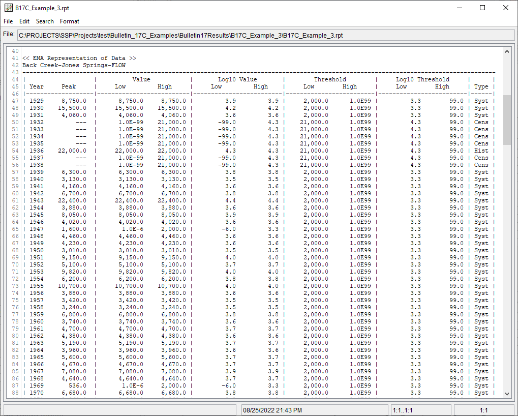
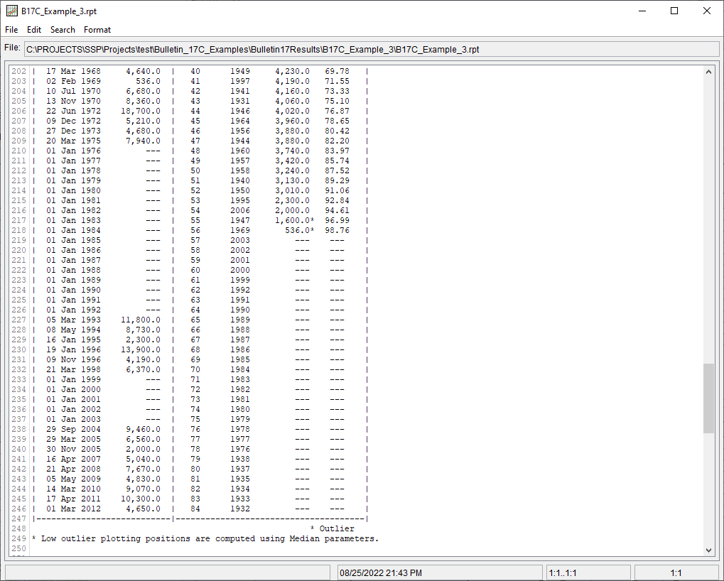
As shown in Figure 4, the Multiple Grubbs-Beck Test identified a low outlier threshold (critical value) of 2000 cfs, which corresponds to the smallest peak that was retained. Two annual peak flows were identified and censored, as shown in Figure 6.  These annual peak flows were then recoded to have a flow interval of zero – 2000. The perception threshold for all systematic observations were also adjusted to correspond with the Multiple Grubbs-Beck Test low outlier threshold (i.e. 2000 – inf), as shown in Figure 7.