Example 4. Historical Data – Arkansas River at Pueblo, CO

Example 4 illustrates the computation of a peak flow frequency curve using EMA and Bulletin 17C procedures with an annual maximum series comprised of systematic and historical flood events as well as paleoflood information. The largest historic floods are described as interval data, and multiple thresholds are needed to effectively extend the discontinued stream gaging record after the dam was built. A paleohydrologic bound of about 840 years (before water year 2004) was estimated at this site for inclusion in the flood frequency curve. No estimates of individual paleofloods were made at this site, due to the relatively wide channel geometry and the lack of apparent stratigraphic evidence of large paleofloods during a limited field study (England, et al., 2018).

When fitting the Log Pearson Type III distribution using either Bulletin 17B or Bulletin 17C procedures, an unregulated annual maximum series is required. However, peak flow rates downloaded from the USGS website do not always reflect unregulated conditions, as is the case with the Arkansas River near Pueblo, CO (07099500) gage. Pueblo Dam, which creates one of the largest reservoirs within Colorado, is immediately upstream of this gaging station. The dam was constructed between 1970 and 1975 and began impacting the annual maximum series due to flood control and water supply storage in water year 1974. As such, the annual maximum series downloaded from the USGS website was altered to reflect unregulated conditions for water year 1974 and 1975. The modified annual maximum series is plotted in Figure 1 and tabulated in Table 1.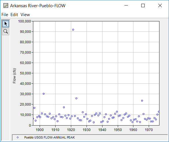


Table 1. Arkansas River near Pueblo, CO Annual Peak Flow Record (Modified).

A Bulletin 17 Analysis using EMA and Bulletin 17C procedures has been developed for this example. To open the analysis, either double-click on the analysis labeled "B17C Example 4" from the Study Explorer or from the Analysis menu select open, then select "B17C Example 4" from the list of available analyses. When "B17C Example 4" is selected, the Bulletin 17 analysis editor will appear as shown in Figure 2. As shown, the Skew option was set to use the Station Skew.

Commonly, within dam safety studies, estimates of flow or volume frequency are required at extremely small exceedance probabilities. As such, additional frequency ordinates (0.1- and 0.01-percent annual chance exceedance probabilities) were specified on the Options tab, as shown in Figure 3. It should be noted that estimating the frequency curve for these probabilities requires extrapolation far beyond the gaged data. However, the inclusion of paleoflood data makes this extrapolation more supportable.

The EMA Data tab for this example is shown in Figure 4. This example uses an annual maximum series consisting of both systematic data along with historical events and paleoflood information. Multiple perception thresholds are needed to reasonably incorporate the various historical and paleoflood information.

• The default "Total Record" perception threshold should be modified to reflect the additional paleoflood and post Pueblo Dam construction information. A start year of 1165 and end year of 2004 along with a perception threshold of zero – inf should be entered on the first line.
• The second perception threshold relates to the non-exceedance information obtained through the paleoflood analysis. A start and end year of 1165 and 1858 should be entered, respectively, along with a 150,000 – inf perception threshold. This implies that no floods exceeded a peak flow rate of 150,000 cfs from 1165 – 1858 even though there were no gages present.
• The third perception threshold represents a period of historical information from 1859 – 1892 where floods in excess of 40,000 cfs would have been recorded had they occurred. Additionally, an historical flow event that occurred in 1864 should be entered in the Flow Ranges table with a low and high flow value of 41,000 and 60,000 cfs, respectively, to denote uncertainty around the best-estimate of 50,500 cfs. The data type for this event should be set to Historical.
• The fourth perception threshold represents an additional period of historical information from 1893 – 1894. A perception threshold of 19,900 – inf should be entered for these two years. Two events that aren't part of the gage record occurred in 1893 and 1894. The 1893 event had a low and high flow value of 20,000 and 25,000, respectively, with a best-estimate of 22,500. The 1894 event had a low and high flow value of 35,000 and 40,000, respectively, with a best-estimate of 37,500. Both events should be entered in the Flow Ranges table and the data types should be set to Historical.
  The 1921 event should be entered as an historical event with uncertainty around the best estimate of 91,500 cfs. A low and high value of 80,000 and 103,000 should be used.
• The fifth and final perception threshold represents the period when the stream gage was discontinued after the construction of Pueblo Dam. It is known that floods in excess of 20,000 cfs would have been recorded had they occurred. Therefore, a perception threshold of 20,000 – inf should be entered for these years.
  Once all five perception thresholds have been entered as shown in Figure 4, click the Apply Thresholds button to assign the complementary flow ranges for the periods of missing data.

Once all of the General and EMA Data tab settings are set or selected, the user can press the Compute button to perform the analysis. Once the computations have been completed, a message window will open stating Compute Complete. Close this window and then select the Tabular Results tab. The analysis window should resemble Figure 5.

In addition to the tabular results, a graphical plot of the computed frequency curves can be obtained by pressing the Plot Curve button at the bottom of the analysis window. The Log Pearson Type III distribution fit using EMA to the input annual maximum flow data set, the 5% and 95% confidence limits, and the computed plotting positions are shown in Figure 6. As is shown, the Log Pearson Type III distribution is well fit to the majority of the data. However, the largest flood event (June 1921) is underfit by the EMA-computed Log Pearson Type III curve. This is likely due to the influence of the paleoflood information which lengthens the historical record from 85 years to 840 years. Consequently, the at-station skew coefficient is reduced which primarily affects the upper end of the computed curve. Had the paleoflood information not been included, a larger at-station skew coefficient would have been computed.