Download PDF
Download page Example 8. [inf – inf] Perception Threshold – Pembina River at Neche, ND.
Example 8. [inf – inf] Perception Threshold – Pembina River at Neche, ND
Example 8 demonstrates how an [inf – inf] perception threshold can be used to compute a peak flow frequency curve using EMA and Bulletin 17C procedures. The use of an [inf – inf] perception threshold for missing years implies that no knowledge is available for those missing years. This produces a result that is equivalent to the elimination of the missing years from the analysis. The data for this example comes from the USGS gage 05100000 Pembina River at Neche, North Dakota. The annual maximum series for this example contains 109 peaks beginning in 1904 and ending in 2016. Two periods of missing data exist within this record, 1909 and 1916-1918. The annual maximum series is plotted in Figure 1 and tabulated in Table 1.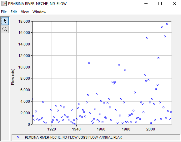
Table 1. Pembina River at Neche, ND Annual Peak Flow Record.
Date | Flow (cfs) |
|---|---|
02 May 1904 | 4300 |
05 Apr 1905 | 1372 |
04 Apr 1906 | 800 |
14 May 1907 | 2190 |
10 Apr 1908 | 927 |
15 Mar 1910 | 685 |
23 Mar 1911 | 900 |
29 Jul 1912 | 1000 |
07 Apr 1913 | 3870 |
18 Apr 1914 | 388 |
07 Apr 1915 | 180 |
15 Apr 1919 | 2430 |
19 Apr 1920 | 361 |
13 Apr 1921 | 733 |
07 Apr 1922 | 1300 |
20 Apr 1923 | 3120 |
20 Apr 1924 | 674 |
28 Mar 1925 | 2350 |
06 Jul 1926 | 318 |
12 May 1927 | 3110 |
25 Mar 1928 | 1270 |
21 Mar 1929 | 750 |
08 Apr 1930 | 2900 |
09 Apr 1931 | 1580 |
09 Apr 1932 | 1240 |
26 May 1933 | 1180 |
09 Apr 1934 | 780 |
18 Jun 1935 | 364 |
15 Apr 1936 | 2530 |
08 Jun 1937 | 237 |
20 Mar 1938 | 730 |
04 Apr 1939 | 52 |
20 Apr 1940 | 816 |
14 Apr 1941 | 2830 |
07 Apr 1942 | 3550 |
27 Mar 1943 | 1400 |
06 Aug 1944 | 1200 |
29 Mar 1945 | 2440 |
24 Mar 1946 | 2070 |
11 Apr 1947 | 1320 |
21 Apr 1948 | 3770 |
22 Apr 1949 | 5010 |
20 Apr 1950 | 10700 |
07 Apr 1951 | 2000 |
03 Apr 1952 | 550 |
10 Jun 1953 | 250 |
07 Jul 1954 | 846 |
05 Apr 1955 | 2700 |
27 Apr 1956 | 5200 |
27 Mar 1957 | 661 |
07 Apr 1958 | 442 |
05 Apr 1959 | 1800 |
14 Apr 1960 | 4040 |
03 Apr 1961 | 372 |
21 Apr 1962 | 3650 |
28 Jul 1963 | 1150 |
17 Apr 1964 | 1080 |
13 Apr 1965 | 3600 |
03 Apr 1966 | 4300 |
23 Apr 1967 | 2900 |
28 Mar 1968 | 734 |
21 Apr 1969 | 7360 |
27 Apr 1970 | 7070 |
12 Apr 1971 | 7350 |
16 Apr 1972 | 2550 |
27 Mar 1973 | 224 |
28 Apr 1974 | 10300 |
18 May 1975 | 1500 |
19 Apr 1976 | 4430 |
21 May 1977 | 261 |
11 Apr 1978 | 3800 |
20 Apr 1979 | 9500 |
07 Apr 1980 | 435 |
01 Apr 1981 | 285 |
08 Jun 1982 | 1520 |
09 Apr 1983 | 1630 |
07 Apr 1984 | 312 |
20 Mar 1985 | 1750 |
24 Mar 1986 | 2390 |
07 Apr 1987 | 5510 |
06 Apr 1988 | 420 |
17 Apr 1989 | 1000 |
03 Apr 1990 | 1000 |
16 Jun 1991 | 888 |
01 Apr 1992 | 3900 |
30 Jul 1993 | 3580 |
02 Apr 1994 | 2040 |
23 Apr 1995 | 8500 |
18 Apr 1996 | 7500 |
27 Apr 1997 | 15100 |
16 Apr 1998 | 7620 |
02 Jun 1999 | 3790 |
22 Mar 2000 | 208 |
22 Apr 2001 | 4420 |
12 Jun 2002 | 3440 |
20 May 2003 | 712 |
01 Apr 2004 | 6120 |
02 Jul 2005 | 6890 |
17 Apr 2006 | 11500 |
30 Mar 2007 | 3800 |
13 Apr 2008 | 847 |
20 Apr 2009 | 16900 |
04 Apr 2010 | 2900 |
19 Apr 2011 | 15300 |
05 Jul 2012 | 991 |
21 May 2013 | 17500 |
13 Apr 2014 | 2300 |
19 May 2015 | 927 |
20 Jul 2016 | 2090 |
A Bulletin 17 Analysis using EMA and Bulletin 17C procedures has been developed for this example. To open the analysis, either double-click on the analysis labeled "B17C Example 8" from the Study Explorer or from the Analysis menu select open, then select "B17C Example 8" from the list of available analyses. When "B17C Example 8" is selected, the Bulletin 17 analysis editor will appear as shown in Figure 2. As shown, the Skew option was set to use the Station Skew.

No changes to the Options tab are necessary. The EMA Data tab for this example is shown in Figure 3. This example uses an annual maximum series consisting of systematic data with two missing periods. The missing periods include 1909 and 1916 – 1918. Since 17C EMA requires a non zero – inf perception threshold for all periods of missing data, a total of three perception thresholds are required. An inf – inf perception threshold is used to convey zero additional knowledge about the missing periods because the complementary flow range for such a perception threshold is zero – inf. Using the aforementioned perception thresholds and flow ranges is equivalent to removing the missing periods of record from the computations. Once all three perception thresholds have been entered as shown in Figure 3, click the Apply Thresholds button to assign the complementary flow ranges for the periods of missing data.

Once all of the General and EMA Data tab settings are set or selected, the user can press the Compute button to perform the analysis. Once the computations have been completed, a message window will open stating Compute Complete. Close this window and then select the Tabular Results tab. The analysis window should resemble Figure 4.

In addition to the tabular results, a graphical plot of the computed frequency curves can be obtained by pressing the Plot Curve button at the bottom of the analysis window. The Log Pearson Type III distribution fit using EMA to the input annual maximum flow data set, the 5% and 95% confidence limits, and the computed plotting positions are shown in Figure 5.

As shown in Figure 6, four years were demarcated using an inf – inf perception threshold (and zero – inf flow range). These annual peak flows were then removed from the EMA computations, as shown in Figure 7.

