Download PDF
Download page Example 9. [0 – value] Perception Threshold – Clark Fork River below Cabinet Gorge Dam, ID.
Example 9. [0 – value] Perception Threshold – Clark Fork River below Cabinet Gorge Dam, ID
Example 9 exhibits how a [0 – value] perception threshold can be used to compute a peak flow frequency curve using EMA and Bulletin 17C procedures. When using a [0 – value] perception threshold, the corresponding flow range spans [value – inf]. For instance, when using a [0 – 5000 cfs] perception threshold, the corresponding flow range would be [5000 cfs – inf]. This implies that the flow for the specified missing years must have exceeded 5000 cfs. The data for this example comes from the USGS gage 12391950 Clark Fork River below Cabinet Gorge Dam, ID. The annual maximum series consists of unregulated daily average flows. The period of record used for this example contains 77 peaks beginning in 1929 and ending in 2008. Two periods of missing data also exist within this record, 1940-1941 and 1944. The annual maximum series is plotted in Figure 1 and tabulated in Table 1.
Table 1. Clark Fork River below Cabinet Gorge Dam, ID Annual Peak Flow Record.
Date | Flow (cfs) |
|---|---|
25 May 1929 | 109495 |
01 Jun 1930 | 66383 |
17 May 1931 | 81758 |
23 May 1932 | 128563 |
17 Jun 1933 | 167893 |
26 Apr 1934 | 110603 |
24 May 1935 | 107358 |
16 May 1936 | 117050 |
29 May 1937 | 71113 |
28 May 1938 | 116598 |
05 May 1939 | 100232 |
28 May 1942 | 99448 |
20 Jun 1943 | 122767 |
03 Jun 1945 | 86562 |
30 May 1946 | 102445 |
10 May 1947 | 156245 |
24 May 1948 | 198024 |
17 May 1949 | 132621 |
23 Jun 1950 | 145329 |
13 May 1951 | 129430 |
29 Apr 1952 | 104365 |
14 Jun 1953 | 131126 |
21 May 1954 | 175076 |
15 Jun 1955 | 117428 |
23 May 1956 | 179458 |
07 May 1957 | 126620 |
26 May 1958 | 123080 |
07 Jun 1959 | 146887 |
05 Jun 1960 | 121354 |
28 May 1961 | 152917 |
30 May 1962 | 96903 |
01 Jun 1963 | 77746 |
10 Jun 1964 | 279802 |
20 Jun 1965 | 128903 |
02 Jun 1966 | 97380 |
24 May 1967 | 150874 |
05 Jun 1968 | 99891 |
15 May 1969 | 105457 |
07 Jun 1970 | 139836 |
14 May 1971 | 145726 |
03 Jun 1972 | 188257 |
20 May 1973 | 83173 |
18 Jun 1974 | 197601 |
21 Jun 1975 | 154409 |
12 May 1976 | 142478 |
04 May 1977 | 49246 |
09 Jun 1978 | 113623 |
27 May 1979 | 124395 |
27 May 1980 | 107620 |
26 May 1981 | 126384 |
17 Jun 1982 | 134238 |
31 May 1983 | 113659 |
01 Jun 1984 | 101039 |
26 May 1985 | 101664 |
01 Jun 1986 | 124274 |
02 May 1987 | 98245 |
15 May 1988 | 65824 |
12 May 1989 | 106999 |
01 Jun 1990 | 105787 |
20 May 1991 | 138662 |
02 May 1992 | 63063 |
16 May 1993 | 110858 |
13 May 1994 | 76657 |
09 Jun 1995 | 94839 |
10 Jun 1996 | 139015 |
18 May 1997 | 209671 |
29 May 1998 | 83841 |
27 May 1999 | 120556 |
25 May 2000 | 80067 |
28 May 2001 | 68919 |
02 Jun 2002 | 136674 |
01 Jun 2003 | 118023 |
08 Jun 2004 | 63594 |
07 Jun 2005 | 73941 |
21 May 2006 | 129591 |
14 May 2007 | 77787 |
21 May 2008 | 154560 |
A Bulletin 17 Analysis using EMA and Bulletin 17C procedures has been developed for this example. To open the analysis, either double-click on the analysis labeled "B17C Example 9" from the Study Explorer or from the Analysis menu select open, then select "B17C Example 9" from the list of available analyses. When "B17C Example 9" is selected, the Bulletin 17 analysis editor will appear as shown in Figure 2. As shown, the Skew option was set to use the Station Skew.

No changes to the Options tab are necessary. The EMA Data tab for this example is shown in Figure 3. This example uses an annual maximum series consisting of systematic data with two missing periods. The missing periods include 1940 – 1941 and 1944. Since 17C EMA requires a non zero – inf perception threshold for all periods of missing data, a total of three perception thresholds are required. In this example, both missing periods make use of a perception threshold of 0 – 50000. This perception threshold implies that had a flow less than 50000 cfs occurred, someone would have measured and recorded it. The complementary flow range for this perception threshold is 50000 – inf. Once all three perception thresholds have been entered as shown in Figure 3, click the Apply Thresholds button to assign the complementary flow ranges for the periods of missing data.

Once all of the General and EMA Data tab settings are set or selected, the user can press the Compute button to perform the analysis. Once the computations have been completed, a message window will open stating Compute Complete. Close this window and then select the Tabular Results tab. The analysis window should resemble Figure 4.

In addition to the tabular results, a graphical plot of the computed frequency curves can be obtained by pressing the Plot Curve button at the bottom of the analysis window. The Log Pearson Type III distribution fit using EMA to the input annual maximum flow data set, the 5% and 95% confidence limits, and the computed plotting positions are shown in Figure 5.
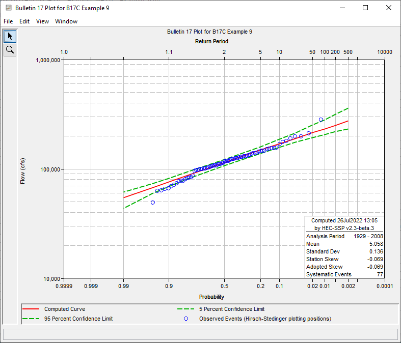
As shown in Figure 6, the perception thresholds for the missing years were encoded as 0 – 50000 while the flow ranges were set to 50000 – inf. This causes the EMA-computed standard deviation and skew absolute value to decrease (compared to the use of inf – inf perception thresholds).
