Example 21. Distribution Fitting, Analyzing a Time Series of Daily Average Flow Using Time Window, Seasonal, and Annual Maxima Filtering

This example demonstrates how to use the Distribution Fitting analysis to analyze a time series of daily average flow using time window, seasonal and annual maxima filtering. The data for this example consists of daily average streamflow for a location along the Sinnemahoning Creek near Sinnemahoning, PA. This stream gage is operated by the USGS (gage ID: 01543500). The period of record used for this example is from 1938 to 2016. To view the data from HEC-SSP, right-click on the data record labeled "Sinnemahoning Creek-Daily" in the study explorer and then select Plot. A plot of the data will appear as shown in Figure 1.

A Distribution Fitting analysis has been developed for this example. A distribution | fitting method combination has not been selected within the SSP Examples study. To visualize, inspect, and select a distribution | fitting method combination, the following steps should be used. To open the Distribution Fitting analysis editor for this example, either double-click on the analysis labeled Distribution Fitting Test 21 from the study explorer, or from the Analysis menu, select open, then select Distribution Fitting Test 21 from the list of available analyses. When this analysis is opened, the Distribution Fitting editor will appear as shown in Figure 2.

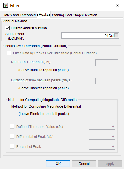
For this analysis, the daily average streamflow data was revised using several filters. First, a Time Window filter was applied spanning 01Oct1939 through 30Sep2015 (i.e. water year 1940 – water year 2015). Second, a seasonal filter was applied spanning 01May – 30Nov (i.e. discard all values outside of this range). Finally, an annual maximum series was extracted using a water year demarcation of 01Oct (i.e. extract annual maxima between 01Oct – 30Sep). Out of the original 28269 values, 76 values remained after data filtering. These 76 values constitute an annual maximum series of daily average streamflow occurring between 01May and 30Nov (i.e. summer and fall months). The filters used within this analysis are shown in Figure 3. The original data as well as the filtered data is shown in Figure 4.

Summary statistics of the original and filtered/processed data can be accessed by pressing the Data Summary Statistics button near the bottom of the Distribution Fitting editor while on the Data tab, as shown in Figure 5.

On the Analysis tab, several analytical distributions and fitting methods are available for selection. As shown in Figure 6, the Filter Using Parameter radio button was selected within the Distribution Filter panel. The default Product Moments fitting method was left unchanged. The default Kolmogorov-Smirnov goodness of fit test was left unchanged. Several analytical distributions (some which poorly fit the data as well as some that fit the data well) were then selected and compared. CDF, PDF, PP, QQ, and CDF-Plotting Position plots comparing these distributions are shown in Figure 7, Figure 8, Figure 9, Figure 10, and Figure 11.

Kolmogorov-Smirnov and Chi-Square summary statistics can be accessed by pressing the Goodness of Fit Summary Statistics button near the top of the Distribution Fitting editor while on the Analysis tab, as shown in Figure 12.

In this example, the Accept Distribution button was selected for the Ln-Normal Distribution using Product Moments. Confidence limits and an expected probability curve were automatically computed using the options specified within the Plot Options and Confidence Limits and Expected Probability Options editors. Specifically, the Log option was selected within the Expected Probability Ordinates panel (which computes the expected probability curve using log base 10 values), the Standard Bootstrap Confidence Limit Type Method was selected, as shown in Figure 13.

The accepted distribution | fitting method was used to populate the Results tab, as shown in Figure 14.

In addition to the tables and plot available on the Results tab, CDF, PDF, and CDF-Plotting Position plots of the data and accepted distribution | fitting method can be obtained by double left-clicking on the plot of interest. The CDF-Plotting Position plot of the data and accepted distribution | fitting method is shown in Figure 15.

In addition to the tabular and graphical results, there is a report file that shows the input data, data filters that were applied, processed data, data summary statistics, all available analytical distributions for the selected fitting method and their corresponding parameters, selected goodness of fit summary scores for each analytical distribution, and the accepted distribution | fitting method. Different types and amounts of information will be contained within the report file depending upon the data and the options that have been selected for the analysis. To review the report file, press the View Report button at the bottom of the analysis window. When this button is selected a text viewer will open the report file and display it on the screen, as shown in Figure 16.