Example 23. Distribution Fitting, Analyzing a Time Series of Daily Precipitation Accumulation Using Peaks Over Threshold Filtering

This example demonstrates how to use the Distribution Fitting analysis to analyze a time series of daily precipitation accumulation using peaks over threshold filtering. The data for this example consists of a daily precipitation accumulation time series for a precipitation gage located near Hawley, Pennsylvania. This precipitation gage is operated by the National Weather Service (NWS). The precipitation data was downloaded from the NWS website ("https://www.ncdc.noaa.gov/") as a comma separated values (.csv) file and ingested to the study using an HEC-DSSVue plugin.  The period of record used for this example is from January 1900 to July 2017. To view the data, right-click on the data record labeled "Hawley 1 E PA-Daily-Precip-Inc" in the study explorer and then select Plot. A plot of the data will appear as shown in Figure 1.

A Distribution Fitting analysis has been developed for this example. A distribution | fitting method combination has not been selected within the SSP Examples study. To visualize, inspect, and select a distribution | fitting method combination, the following steps should be used. To open the Distribution Fitting analysis editor for this example, either double-click on the analysis labeled Distribution Fitting Test 23 from the study explorer, or from the Analysis menu, select open, then select Distribution Fitting Test 23 from the list of available analyses. When this analysis is opened, the Distribution Fitting editor will appear as shown in Figure 2.

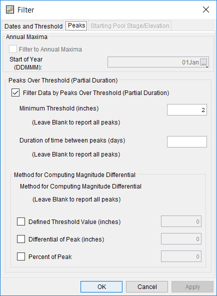
For this analysis, the daily precipitation data was revised using several filters. First, a Time Window filter was applied spanning 01Oct1921 through 30Sep2017 (i.e. water year 1922 – water year 2017). Second, peaks were extracted from the remaining daily precipitation accumulations using a minimum threshold of 2 inches. Out of the original 31383 values, 121 values remained after data filtering. These 121 peak values constitute a partial duration series of daily precipitation accumulations in excess of 2 inches. The filters used within this analysis are shown in Figure 3. The original data as well as the filtered data is shown in Figure 4.

Summary statistics of the original and filtered/processed data can be accessed by pressing the Data Summary Statistics button near the bottom of the Distribution Fitting editor while on the Data tab, as shown in Figure 5.

On the Analysis tab, several analytical distributions and fitting methods are available for selection. As shown in Figure 6, the Display All Distributions radio button was selected within the Distribution Filter panel to display all of the available analytical distributions. The L-Moments Fitting method was selected. The default Kolmogorov-Smirnov goodness of fit test was left unchanged. Several analytical distributions (some which poorly fit the data as well as some that fit the data well) were then selected and compared. CDF, PDF, PP, QQ, and CDF-Plotting Position plots comparing these distributions are shown in Figure 7, Figure 8. Figure 9, Figure 10, and Figure 11.

Kolmogorov-Smirnov and Chi-Square summary statistics can be accessed by pressing the Goodness of Fit Summary Statistics button near the top of the Distribution Fitting editor while on the Analysis tab, as shown in Figure 12.

In this example, the Generalized Pareto Distribution fit using L-Moments was selected by clicking the Accept Distribution button. Upon clicking this button, confidence limits and an expected probability curve were automatically computed using the options specified within the Plot Options and Confidence Limits and Expected Probability Options editors. The default confidence limits options were selected, as shown in Figure 13.  

The accepted distribution | fitting method was used to populate the Results tab, as shown in Figure 14.

In addition to the tables and plot available on the Results tab, CDF, PDF, and CDF-Plotting Position plots of the data and accepted distribution | fitting method can be obtained by double left-clicking on the plot of interest. The CDF-Plotting Position plot of the data and accepted distribution | fitting method is shown in Figure 15.

In addition to the tabular and graphical results, there is a report file that shows the input data, data filters that were applied, processed data, data summary statistics, all available analytical distributions for the selected fitting method and their corresponding parameters, selected goodness of fit summary scores for each analytical distribution, and the accepted distribution | fitting method. Different types and amounts of information will be contained within the report file depending upon the data and the options that have been selected for the analysis. To review the report file, press the View Report button at the bottom of the analysis window. When this button is selected a text viewer will open the report file and display it on the screen, as shown in Figure 16.