Download PDF
Download page Applying the Variable Time Window Option in a Bulletin 17 Analysis.
Applying the Variable Time Window Option in a Bulletin 17 Analysis
Overview
This tutorial provides an example application of the Variable Time Window option within the Bulletin 17 Analysis. The variable time window option is a way to explore how individual flood peaks impact a flow-frequency curve as well as the parameters of the Log Pearson Type III Distribution. The variable time window option should not be used when computing final, project specific, flow-frequency curves.
HEC-SSP version 2.3.1 was used to create this example. You will need HEC-SSP version 2.3.1, or newer, to open the project files.
Download a copy of the initial HEC-SSP project here:

Introduction
When performing flow-frequency analysis, the mean, standard deviation, and skew coefficients are estimated from a sample of annual maximum series. The skew coefficient estimated from the sample, referred to as the station skew, is particularly difficult to estimate accurately as it is sensitive to outliers. The estimated skew coefficient for short records may not provide an accurate representation of the true population skew coefficient. In this task, the Expanding Window Analysis and Moving Window Analysis will be used to explore the effect of sample size on estimating station skew.
The Moving Window Analysis computes the Bulletin 17 analysis using a fixed computational window, and increments the window by a specified number of years for each calculation. For example, if the period of record of the analysis is 1925–2010, and a moving window of 30 years incremented by 1 year is used, a Bulletin 17 analysis would first be performed for the 30-year period from 1925–1954. Then, a Bulletin 17 analysis would be performed for the 30-year period from 1926–1955, and so on, until the end of the period of record is reached.
The Expanding Window Analysis computes the Bulletin 17 analysis using a computational window that increases by a specified number of years for each calculation. For example, if the period of record of the analysis is 1925–2010, and an expanding window starting at 30 years and incremented by 1 year is used, a Bulletin 17 analysis would first be performed for the 30-year period from 1925–1954. Then, a Bulletin 17 analysis would be performed for the 31-year period from 1925–1955, and so on, until the end of the period of record is reached.
Bulletin 17 Analysis
Open the example HEC-SSP project. As shown below, there is one dataset in the project and a Bulletin 17 analysis named Base Analysis. The Bushkill Creek at Shoemakers, PA stream gage is located in Eastern Pennsylvania.

The figure below shows annual maximum peak flows from 1909 through 2019 (there are 111 measured flood events). Notice the extreme event in 1955. Peak flow for the 1955 event was 23,400 cfs; whereas, the next largest flood was 7,300 cfs in 1969.

A common question when evaluating a flow-frequency analysis is: how impactful are certain large events to the computed flow-frequency curve? You can imagine that including the 1955 event would result in a large positive skew value. To investigate this question, begin by opening the Base Analysis Bulletin 17 Analysis. The Base Analysis uses the Bush Kill annual maximum peak flows and the 17C EMA method to compute the flow-frequency curve. All default options were selected in the 17C EMA analysis. The Use Station Skew, Do Not Compute Expected Probability Curve, and Default Confidence Limits options were selected on the General tab. No Low Outlier Threshold was entered and the Do Not Compute Using Variable Time Window option was selected on the General tab. The figure below shows the EMA Data tab, no historic events or periods outside the range of systematic data were defined.

The figure below shows the computed frequency curve plot. Notice the 1955 flood event plots significantly above the computed curve. Ideally, the modeler would investigate additional flood information in an attempt to place this flood event in a longer context; it is likely that this event is much rarer than its empirical plotting position of approximately 1/100 leads you to believe. For this tutorial, we will explore how the 1955 flood impacts the Log Pearson Type III distribution parameters and computed flow-frequency information using the Variable Time Window option.

Moving Window Option
- Create a copy of the Base Analysis by selecting the analysis name in the tree, clicking the right mouse button, and selecting the Save As option. Enter a name of Moving Average and click the OK button.

- Double click the Moving Average analysis name to open the Bulletin 17 Editor.
- Go to the Options tab. Within the Variable Time Window panel, click the Compute Using Moving Window radio button. Change the Window Length to 30 years and the Shift Increment to 1 year.

- Click the Compute button. The compute should take between 15 and 20 seconds to complete.
The results are located in the Variable Time Window Results tab. Under the Flow tab, the estimated flow for the given percent chance exceedances are shown for each computation window. The Statistics tab shows the mean, standard deviation, and skew coefficients for each computation window.
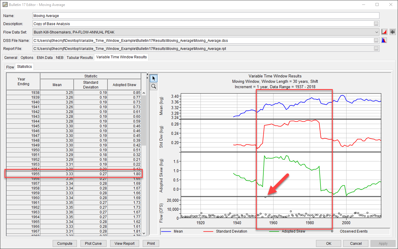
- Go to the Variable Time Window Results tab and then select the Statistics tab. The results show how the computed mean, standard deviation, and skew vary as the 30 year analysis period was shifted throughout the overall time window. 1938 is the first year with 30 years of data. Notice how the standard deviation and skew change drastically when the large flood event in 1955 was included. Elevated standard deviations and skews are realized until 1986, which is when the 1955 event dropped out of the computation. The results indicate that the 1955 flood event has a large impact on an analysis with just 30 years of flow data.
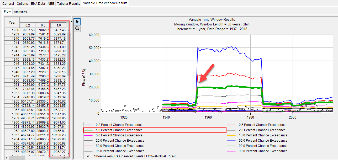
- Open the Flow tab, as shown below. Results on this tab show how the computed flow-frequency information changes for each 30 year window. The green line is the 1-percent flow estimate for each 30 year window. Notice how the 1-percent flow estimate jumps from approximately 6000 cfs for the period 1925-1954 to nearly 20000 cfs for the period 1935-1955. The estimated 1-percent flow is reduced after the 30 year analysis window no longer includes the 1955 event. Also, notice how the 1955 event has lesser impacts on the 10 through 99-percent flow estimates.
Bulletin 17 Results
When using the Moving Window option, note that results on the Tabular Results tab and in the Plot only reflect results from the final moving window. The results are not for the entire analysis window defined on the EMA Data tab.
Expanding Window Option
- Create a copy of the Base Analysis by selecting the analysis name in the tree, clicking the right mouse button, and selecting the Save As option. Enter a name of Expanding Window and click the OK button.

- Double click the Expanding Window analysis name to open the Bulletin 17 Editor.
- Go to the Options tab. Within the Variable Time Window panel, click the Compute Using Expanding Window radio button. Change the Initial Window Length to 30 years and the Expansion Increment to 1 year.

- Click the Compute button. The compute should take between 45 and 50 seconds to complete.
The results are located in the Variable Time Window Results tab. Under the Flow tab, the estimated flow for the given percent chance exceedances are shown for each computation window. The Statistics tab shows the mean, standard deviation, and skew coefficients for each computation window.
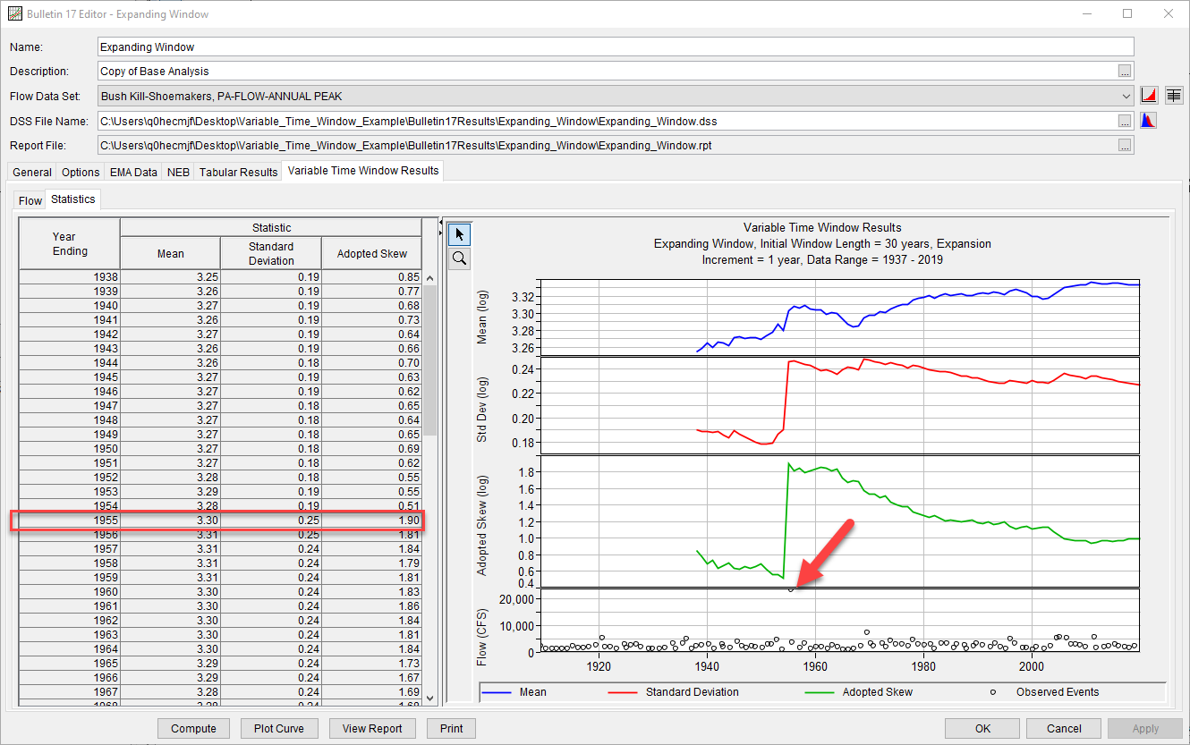
- Go to the Variable Time Window Results tab and then select the Statistics tab. The results show how the computed mean, standard deviation, and skew change as each flow value is added to the computation. 1938 is the first year with 30 years of data. The computation for 1939 includes 31 years of data and the computation for 1940 includes 32 years of data, etc. Notice how the standard deviation and skew change drastically when the large flood event in 1955 was added to the computation. The standard deviation does not change much after 1955, but the skew estimate gradually becomes smaller as more flow values are added to the computation.
- Open the Flow tab, as shown below. Results on this tab show how the computed flow-frequency information changes as more flow values are added to the computation (the first computation has only 30 flow values and the final computation has 111 flow values). The green line is the 1-percent flow estimate for each analysis period. Notice how the 1-percent flow estimate jumps from approximately 6200 cfs for the period 1909-1954 to over 15000 cfs for the period 1909-1955. The estimated 1-percent flow is reduced as additional flow values are added to the analysis.
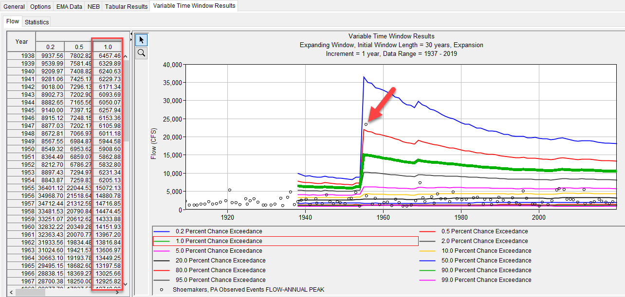
While a period of record of 111 years is considered long by many hydrological standards, the estimates of the mean, standard deviation, and skew coefficient still appear volatile and have not yet converged. Estimating these parameters is difficult and would require thousands of years of data to accurately estimate the population statistics. This highlights the large amount of uncertainty inherent in flow-frequency analyses as well as the importance of including as much additional information (such as historical floods) as possible.