Incorporation of Regional Skew

Overview

When using EMA and incorporating regional skew information, previous versions of EMA could incorrectly weight the regional skew information.  This was corrected in version 2.3 by implementing Equation 7-10 from Bulletin 17C (England et al, 2019).

This correction WILL affect the parameterization of the distribution (i.e. mean, standard deviation, and skew), confidence limits, and quantile variance when incorporating regional skew information.  Users are strongly encouraged to update any analyses that incorporated regional skew information to take advantage of these improved techniques.

Background

The use of regional skew information within Federal flood-frequency guidelines dates to Bulletin 17, which included a procedure for weighting at-site skew and a regional skew (Water Resources Council, 1976). Tasker showed that the minimum variance skew estimator would be obtained by weighting at-site and regional skews by the inverse of their variances (Tasker, 1978). Bulletin 17B  (B17B) recommended the use of an inverse MSE weighting scheme to reflect estimator bias (Interagency Advisory Committee on Water Data, 1982). This B17B weighting scheme is expressed as:

$//<![CDATA[ \begin{array}{l}\tilde{G}=\frac{M S E_{\hat{\gamma}} * G+M S E_{G} * \hat{\gamma}}{M S E_{\hat{\gamma}}+M S E_{G}}\end{array} //]]>$ (1)

where $//<![CDATA[ \begin{array}{l}\hat{\gamma}}\end{array} //]]>$ = at-site skew, $//<![CDATA[ \begin{array}{l}G\end{array} //]]>$ = regional skew, $//<![CDATA[ \begin{array}{l}M S E_{\hat{\gamma}}\end{array} //]]>$ = mean-square error of the at-site skew, $//<![CDATA[ \begin{array}{l}M S E_{G}}\end{array} //]]>$ = mean-square error of the regional skew, and $//<![CDATA[ \begin{array}{l}\tilde{G}\end{array} //]]>$ = weighted skew.

Equation 1 has been shown to minimize the MSE of the skew estimator so long as the regional skew, G, is unbiased and independent of the at-site skew estimator (Griffis and Stedinger, 2009). Equation 1 is simply a weighted average of two independent random variables.

HEC-SSP version 2.2 utilized the following procedure from Appendix 7 in Bulletin 17C (England et al., 2019) to fit the LPIII distribution given a regional skew estimate:

1. Estimate at-site skew
   1. Estimate LPIII parameters using Equations 7-1, 7-2, and 7-3 from Bulletin 17C
   2. Test for convergence
      1. If not converged, return to step 1a
      2. If converged, record the at-site LPIII parameters and move on to step 2
2. Estimate weighted skew
   1. Estimate LPIII parameters using Equations 7-1, 7-2, and 7-3 from Bulletin 17C
   2. Estimate a weighted skew coefficient using Equation (1)
   3. Test for convergence
      1. If not converged, return to step 2a
      2. If converged, record the final LPIII parameters

The above procedure lead to erroneous results when 1) the at-site and regional skew estimates differ by an appreciable amount or 2) many EMA iterations are required for convergence with a regional skew. In general, more EMA iterations are needed when large amounts of historical and censored data are included. The error occurs because a new weighted skew estimate is calculated after each EMA iteration in Step 2b. The at-site skew estimate for the current EMA iteration is influenced by the weighting that took place in the previous EMA iteration. This means the at-site skew estimates for the 2nd and all subsequent EMA iterations are no longer an independent at-site skew value and should not be used in Equation (1). The current procedure results in an overweighting of the regional skew that compounds with each additional EMA iteration. Additionally, the weights were assigned to the wrong terms within Equation (1).

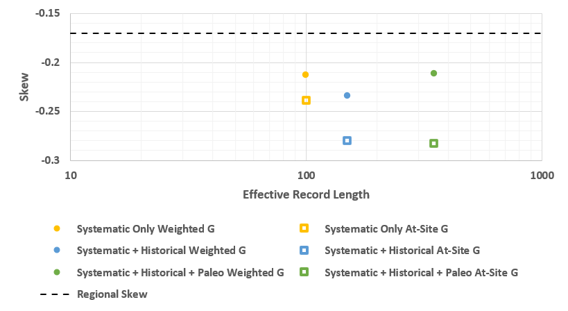
The issue was discovered during a recent flow-frequency analysis that utilized systematic, historical, paleoflood, and regional skew information. The evolution of the at-site and weighted skew estimates is shown in the following figure for analyses that included systematic only, systematic + historical, and systematic + historical + paleoflood information. As more at-site information was added to the analysis (reflected by an increase in the ERL of the parameterized distribution), the at-site skew should decrease and the weighted skew estimate (solid circles) should have trended toward the at-site skew estimate (open squares). Instead, the weighted skew estimate trended in the opposite direction toward the regional skew estimate (dashed line) due to the overweighting of the regional skew. For reference, the regional skew of -0.17 had an associated $//<![CDATA[ \begin{array}{l}M S E_{G}}\end{array} //]]>$ of 0.12.

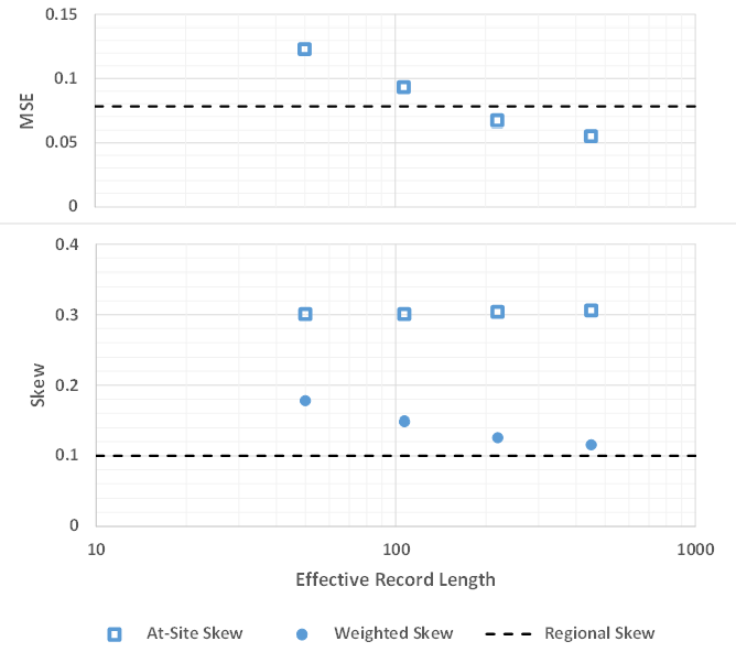
The issue can also be demonstrated by experiment using synthetic datasets having fixed parameters and varying amounts of historical and censored data. Four sample datasets were generated using 50 years of systematic data and increasing amounts of historical information in order to generate LPIII distributions with a mean (of logs) of 4.0, standard deviation (of logs) of 0.3, and at-site skew (of logs) of 0.3. These distributions had ERLs of 50, 110, 220, and 450 years. A regional skew value of 0.1 with an $//<![CDATA[ \begin{array}{l}M S E_{G}}\end{array} //]]>$ of 0.078 was assumed for all four datasets. The following figure shows the evolution of the MSE and weighted skew estimate (solid circles) for each dataset.

The results shown in the above figures demonstrate a similar behavior: the weighted skew coefficients obtained using the current implementation of EMA generally trend toward the regional skew coefficient as ERL of the parameterized distribution increases. This result is counterintuitive and violates the first principles embodied in Equation (1). As the ERL of the parameterized distribution increases, the information content of the at-site skew estimator increases while the information content of the regional skew information remains the same. This means that the influence of regional skew on the weighted skew estimate should decrease with increasing at-site ERL. However, this behavior is not realized using the current procedure. The magnitude of the error is primarily a function of the number of EMA iterations which generally increases with increasing ERL when historical and censored data is included.

Improvements to Weighted Skew Computations

Griffis et al, improved the estimation of the third moment within EMA by directly incorporating regional skew information (Griffis, Stedinger, & Cohn, 2004).

Their algorithm is represented in Bulletin 17C as Equation 7-10.  The improvement is presented here as Equation (2), which when combined with Equation 7-3 within Bulletin 17C, is equivalent to Equation 7-10 within Bulletin 17C.  It is key to weight the skew estimators by the appropriate record lengths:

$//<![CDATA[ \begin{array}{l}\hat{\gamma}_{i}=\frac{\left(G * N_{G}\right)+\left(\hat{\gamma}_{i-1} * N_{T}\right)}{N_{T}+N_{G}}\end{array} //]]>$ (2)

where $//<![CDATA[ \begin{array}{l}\hat{\gamma}_{i}\end{array} //]]>$ = weighted skew for the current iteration, $//<![CDATA[ \begin{array}{l}\hat{\gamma}_{i-1}\end{array} //]]>$ = weighted skew from the previous iteration, $//<![CDATA[ \begin{array}{l}G\end{array} //]]>$ = regional skew, $//<![CDATA[ \begin{array}{l}N_{G}\end{array} //]]>$ = relative effective record length of the regional skew (years), and $//<![CDATA[ \begin{array}{l}N_{T}\end{array} //]]>$ = total record length (years).  $//<![CDATA[ \begin{array}{l}N_{G}\end{array} //]]>$ is computed using a combination of Equation 2 and Equation 16 from Griffis, Stedinger, and Cohn (2004).

HEC-SSP version 2.3 has been modified to use Equation (2) when incorporating regional skew information within a Bulletin 17C compute.  The use of Equation (2) ensures that the weighted skew corresponds to the adjusted mean and standard deviation fit to the data (Griffis, Stedinger, and Cohn, 2004), and eliminates the incorrect weighting of the regional skew information that occurs with the current procedure. Specifically, HEC-SSP version 2.3 utilizes the following procedure to fit the LPIII distribution given a regional skew estimate:

1. Estimate at-site skew
   1. Estimate LPIII parameters using Equations 7-1, 7-2, and 7-3 from Bulletin 17C
   2. Test for convergence
      1. If not converged, return to step 1a
      2. If converged, record the at-site LPIII parameters and move on to step 2
2. Estimate weighted skew
   1. Estimate n_G
   2. Estimate LPIII parameters using Equations 7-1, 7-2, and 7-10 from Bulletin 17C
   3. Test for convergence
      1. If not converged, return to step 2b
      2. If converged, record the final LPIII parameters

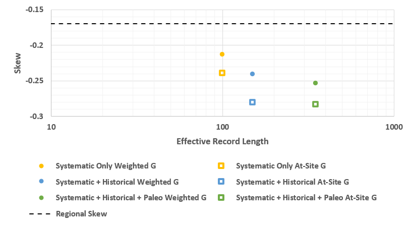
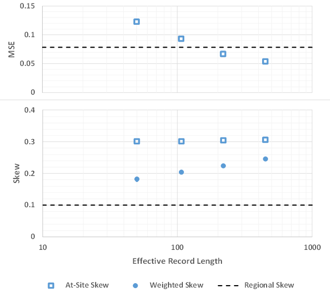
The above procedure eliminates the use of Equation (1) and replaces the use of Equation 7-3 with Equation 7-10 from Bulletin 17C.  The previously described examples were used to demonstrate the improvement with the proposed procedure. The results are shown in the following figures.  

The weighted skew coefficients obtained using the proposed procedure incorporate a correct implementation of EMA as described within Bulletin 17C and exhibit the correct behavior trending toward the at-site skew coefficient as the ERL of the parameterized distribution increases and the at-site skew MSE decreases.