Download PDF
Download page Plotting Positions for Interval Data.
Plotting Positions for Interval Data
Overview
Previous versions of HEC-SSP calculated Hirsch/Stedinger plotting positions for interval data (i.e. low value not equal to the high value) using the geometric mean, or log-average, of the user specified low and high flow values. Specifically, the geometric mean was used to determine if an interval flood was above or below a given threshold and to determine the rank of the flood. Use of the geometric mean lacked transparency and created an interdependence between plotting position and distribution fitting forcing users to make tradeoffs between the two. These situations were most commonly encountered when using paleoflood data which can include evidence (or lack of evidence) of pre-historic floods. The Hirsch/Stedinger plotting position computations have been modified such that the user-specified flow magnitude (as entered within the Peak column) will be used to determined whether the flood is above or below a threshold and to index the flood.
This change only affects the computed plotting positions for interval data. The parameterization of the distribution (i.e. mean, standard deviation, and skew), confidence limits, and quantile variance will be unaffected by these changes.
Plotting Positions
Empirical exceedance probability estimates for observed annual maxima are made using plotting positions. A generic plotting position formula for systematic (exact) observations can be expressed as (U.S. Army Corps of Engineers, 2021):
| 1) | P=\frac{(i-A)}{(n+1-2A)} |
where Pi = exceedance probability of the ith observed annual maxima, i = rank of observed annual maxima from largest (i = 1) to smallest (i = n), n = number of observed annual maxima, and A = constant.
An empirical probability distribution results from the application of Equation 1. Empirical distributions can be used to visually assess the fit of a parameterized analytical distribution such as Log Pearson Type III. When historical and censored data are included, an alternative plotting position methodology is needed. Hirsch and Stedinger (1987) developed a method to compute plotting positions for censored data. They emphasized the correct interpretation of the information conveyed by historical flood data, the recognition of the limited precision of estimates of the exceedance probabilities of historical floods, and showed that any estimator will be somewhat imprecise (Hirsch & Stedinger, 1987).
Bulletin 17C recommends use of the Hirsch-Stedinger threshold exceedance plotting position procedure (England, et al., 2019). The formula for floods exceeding a single perception threshold is expressed as:
| 2) | P=\frac{(k)}{(n)}\frac{(i-A)}{(n+1-2A)} |
where Pi = exceedance probability of the ith above threshold observed annual maxima, I = rank of the above threshold floods from largest (i = 1) to smallest (i = k), k = number of floods above the threshold, and n = total record length including the threshold.
HEC-SSP uses Equation 2 to calculate plotting positions for above and below threshold floods given one or more thresholds.
Within HEC-SSP version 2.2, for historical flow interval data, the geometric mean (or log-average) of the user specified low and high flow values was used to determine if a flood is above or below a given threshold and to determine the rank of a flood. The geometric mean, \bar{Q}_{i}, for a flow interval was computed as:
| 3) | \bar{Q}_{i}=\sqrt{\left(Q_{i, l}\right)\left(Q_{i, u}\right)} |
where Q_{i, l} = the low value of the flow interval and Q_{i, u} = the high value of the flow interval.
Example
Use of the geometric mean lacked transparency and created an interdependency between plotting position and distribution fitting that forced users to make a tradeoff. Tradeoffs are commonly encountered when using paleoflood data, which can include evidence of a pre-historic flood called a paleostage indicator (PSI) or evidence of an absence of flooding called a non-exceedance bound (NEB). Flow intervals are typically used to model a PSI with a corresponding perception threshold. Perception thresholds are typically used to model a NEB. The interdependency occurs because both the parameter and plotting position estimates are a function of the low and high flow values. In certain cases, the user must manipulate the low and high values or the corresponding perception threshold value to obtain the desired plotting position which could have an adverse impact on the parameter estimates.
Consider the example shown in the table below where there is geologic evidence of a PSI. Both the age and discharge needed to define the PSI and corresponding perception threshold are uncertain due to various geologic and hydraulic uncertainties.
Feature | Age (years before present) | Discharge (cfs) | ||
|---|---|---|---|---|
PSI | Young | 1100 | Low | 275,000 |
Best Estimate | 1500 | Best Estimate | 375,000 | |
Old | 1800 | High | 425,000 | |
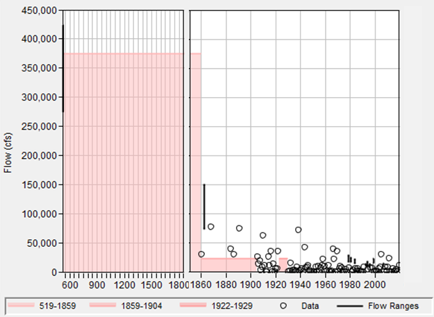
The PSI was included within a flow-frequency analysis as a flow interval observation spanning 275,000 to 425,000 cfs. A best estimate perception threshold was included as a perception range spanning 375,000 cfs to infinity. The perception threshold was applied over a historical period corresponding to the best estimate age of the PSI. A chronology plot of this information is shown in the following figure.

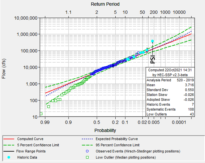
Computing the flow-frequency analysis using the current procedure resulted in the information contained within the following figure. Of particular importance is the computed plotting position for the PSI, which has an AEP on the order of 0.005 (200-year return period).
This result occurs because the geometric mean of the PSI flow interval (342,000 cfs) is less than the perception threshold (375,000 cfs). The plotting position conflicts with the knowledge that the PSI exceeded all thresholds over the 1500-year period of analysis. To obtain the correct plotting position, the user must modify the perception threshold value or the PSI flow interval values so that the geometric mean of the PSI interval is greater than the threshold. However, these modifications would conflict with the best estimates and would change the parameter estimates.

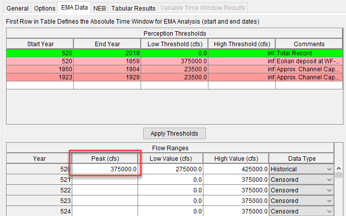
Within version 2.3, user's can specify a flow magnitude to determine if a flood represented by a flow interval is above or below a threshold and to rank the flood. This is accomplished within the EMA Data tab, as shown in the following figure.

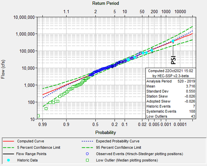
Recomputing the flow-frequency analysis with a specified flow value of 375,000 cfs for the PSI results in the information contained within the following figure. The resultant plotting position of the PSI now has an AEP on the order of 0.0003 (1 in 3000-year return period) consistent with the available information.

The parameterized LPIII distribution, confidence limits, and expected probability curves are unaffected by this change. Only the plotting positions are affected. This gives the user more transparency and control to obtain the desired plotting positions without needing to manipulate inputs that affect the parameter estimates.