Using a Correlation Analysis to Select a Suitable Nearby Gage for Record Extension

Overview

This tutorial provides an example application of the new Correlation Analysis. The correlation analysis is a way to explore how closely related the flows are at nearby gage locations. HEC-SSP version 2.3 beta.1 was used to create this example. 

Download a copy of the initial HEC-SSP project here – Correlation_Analysis_Example_Initial.zip

Introduction

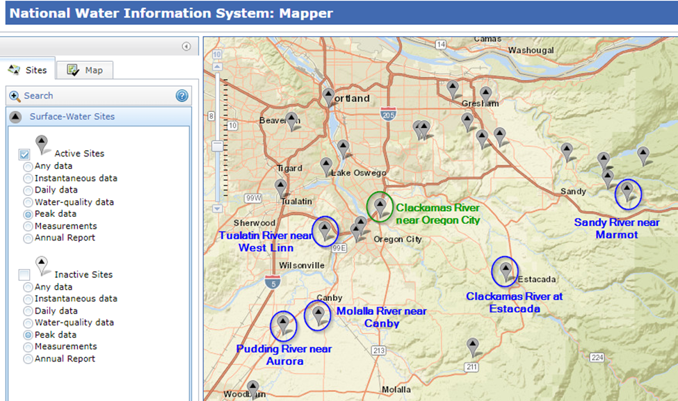
Open the example HEC-SSP project. In this example, the gage location of primary interest is USGS 14211010, Clackamas River near Oregon City. It only exists for about 20 years from 2001-2020, but nearby gages with more years of data can be used to extend the record. The correlation analysis here will help decide which gages are best for record extension. To identify potential candidate sites, the USGS NWIS mapper (https://maps.waterdata.usgs.gov/mapper/index.html) was browsed to find gages geographically nearby with fairly comparable drainage areas. The correlation analysis should be performed on datasets with peak flow records unaffected by upstream regulation. The Tualatin River has a flood risk management project far upstream that is assumed to have a nearly negligible effect at West Linn, so it is kept as a candidate site. If there are nearby sites that are affected by upstream regulation, an unregulated dataset that strips out the upstream regulation effects would be computed and used for the correlation analysis.

As shown below, there are 6 datasets in the project in northwestern Oregon. It is fairly clear in this example that the Clackamas River at Estacada gage should have the best correlation to the Clackamas River near Oregon City gage. However, the choice is not always so obvious. This example will help show how well flow measurements at the Clackamas River near Oregon City gage is to the other nearby gages.

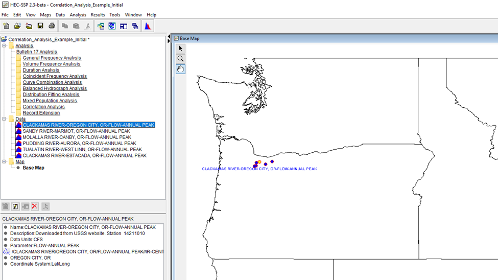
The figure below shows the HEC-SSP project and the location of the six flow gages. 

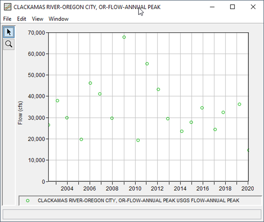
The figure below shows annual maximum peak flows from 2001 through 2020 from the Clackamas River near Oregon City gage.  Notice there do not appear to be any extremely large floods during this period that stand out well above the rest of the dataset. 

Create the Correlation Analysis

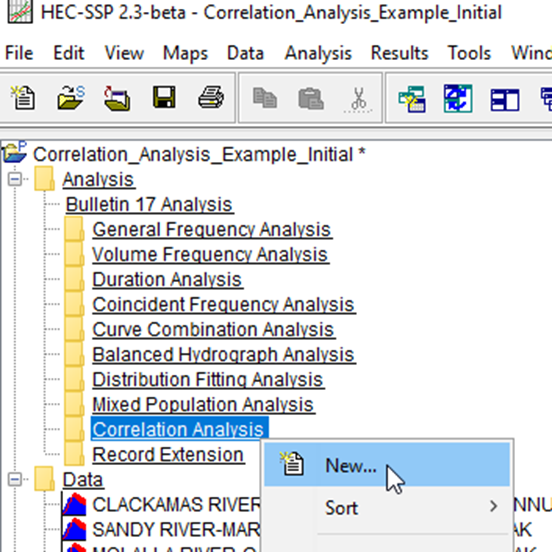
1. Create a new Correlation Analysis by right clicking on the folder in the tree and selecting New. Enter a name for the Correlation Analysis.
   
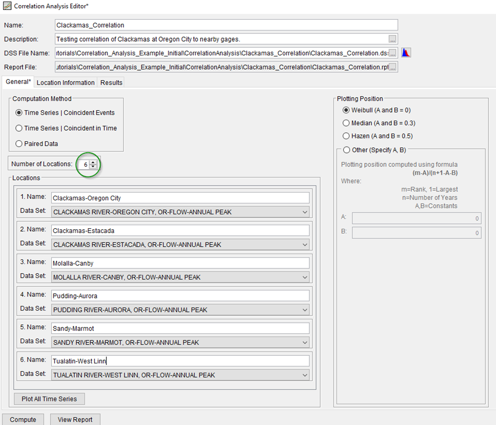
2. Change the Number of Locations to 6.
3. Under the Locations heading, use the drop down menus to select the 6 datasets. Provide a name for each of the datasets. The resulting window should look something like below.
   
    
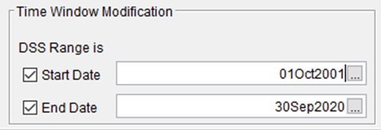
4. At the bottom right of the General tab, under the Time Window Modification heading, change the time window. Change the Start Date to 01Oct2001, and the End Date to 30Sep2020. We are only interested in this time window since the dataset at Clackamas River near Oregon City gage only has data for 19 water years from 2002-2020. If this Time Window Modification step is not taken, the correlation analysis will still compute. However, it will generate warning messages that inconsistent record lengths were supplied for the various datasets. 
   
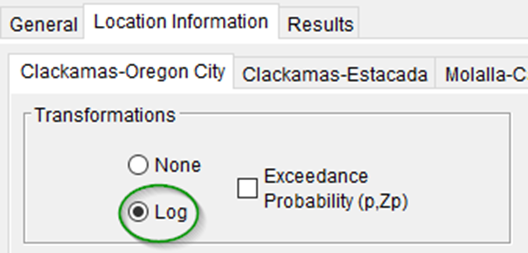
5. Go to the Location Information tab. Each site is displayed as a tab. With annual maximum peak flow datasets, typically correlations are computed on the logarithms of the peak flows. Under the Transformations heading, select Log for all of the 6 datasets. If the correlation analysis is being performed on a different type of variable, such as stage, no transformation would be applied. The Exceedance Probability (p, Zp) option would typically be used if the computed correlations were intended to be used in a Monte Carlo Sampling scheme. Since this example is only a screening analysis to compare the correlations between multiple sites, a log transformation alone is sufficient.
   
    
6. Enter a Typical Event Length (days) of 5 days for all sites. If the annual maximum peak flows occur more than 5 days apart between two of the locations, HEC-SSP will assume that these peak flow records came from different flood events and will not use them when calculating the correlation.
7. Press Compute. Note the warning messages about which events were dropped from the analysis because the date of peak flow was too far apart.
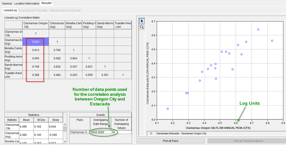
8. Go to the Results tab. The computed correlation matrix between all sites is shown below. As expected, the Clackamas at Estacada site has the highest correlation with the Clackamas River near Oregon City gage. In addition, all 19 years of data were used to compute the correlation, meaning that the peak flow at Estacada was always within a few days of the peak flow at Clackamas River near Oregon City gage. The Molalla River at Canby also has a very strong correlation, since the Mollala River watershed is immediately adjacent to the Clackamas River. However, only 16 of the 19 total years had peak flows coincident in time with the Molalla River gage. While the Pudding River and Tualatin River gages are geographically close to the Clackamas River, the watershed areas are farther from the Clackamas and the correlation is weaker.
   
    

Download a copy of the final HEC-SSP project here - Correlation_Analysis_Example_Final.zip