Task 6. Create a Volume Frequency Analysis and Develop a Family of Volume-Frequency Curves

Download the data file here: DailyAverage_Obs_Data.dss

Import Daily Average Flow Data

• Click Data | New | Using Import Wizard…
• Do not modify anything on the first panel.
• Click the Next button.
• Select HEC-DSS as the source location and click the Next button.
• Within the Selected DSS File row, click the ellipsis button.
• Navigate to the “DailyAverage_Obs_Data.dss” file.
• Select the SAYERS time series that is contained within this file by double left-clicking to add it to the window at the bottom of the Data Importer.
• Click Next and review your data one last time.
• When ready, click Import to to import the data set and return to the main HEC-SSP desktop.
• Click the Save button () to save the study.
• You should notice that a new record was added to the Study Explorer window under Data that contains the daily average inflow time series for Sayers Dam.

Perform a Volume-Frequency Analysis for Sayers Dam

Next, you will develop a family of volume-frequency curves using the Volume-Frequency analysis.  Within this analysis, volume-duration data will be extracted from the daily average inflow time series for multiple durations and LPIII analytical distributions will be subsequently fit using EMA.

• Begin by selecting Analysis | New | Volume-Frequency Analysis.
• Name the new analysis “SayersDam_VDF” and add an adequate description.
• Click the Flow Data Set drop down menu and select the available record.

Only regular records (e.g. those with an E-Part of 1DAY) will be available within this drop down menu.

• Click the Plot Yearly Data button within the Year Specification
  • This will create a Year-Over-Year plot which contains all the data overlaid on top of one another using an x-axis that spans exactly one year beginning with the selected water year, as shown in the following figure.
  • The analyst should decide whether the water year, calendar year, or some other date should be used when extracting the duration data and performing the analysis.

• The General tab should look similar to the following figure.

Question:  When do large flood events tend to occur within the Bald Eagle Creek watershed?  What is an appropriate Year Specification for this location?

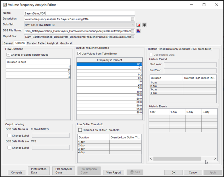
• Move to the Options
• Toggle the ability to define more values within the Flow Durations
• Enter the 1-, 2-, 3-, and 4-day
• Delete the two unnecessary rows.

The durations chosen for this analysis should correspond to the critical duration for the specific project in question.  In order to provide adequate definition around the critical duration, multiple durations less than/greater than the critical duration were chosen.

• Toggle the ability to define more values within the User Specified Frequency Ordinates table.
• Right-click within the table and add an additional three rows.
• Within the new rows, add the 0.1-, 0.01-, and 0.001-percent frequency ordinates.
  • This corresponds to the 1/1000, 1/10,000, and 1/100,000 AEP.
• The Options tab should look similar to the following figure.

• Move to the Duration Table
  • Notice that AMS for the 1-, 2-, 3-, and 4-day durations have been extracted and placed within this table.
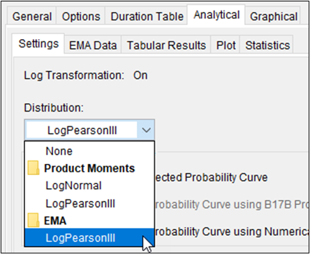
• Move to the Analytical | Settings
• Within the Distribution drop down menu, select the LogPearsonIII | EMA option, as shown in the following figure.
  • This will automatically select other features including the Multiple Grubbs-Beck low outlier test and Hirsch/Stedinger plotting positions (on the General tab).

• Select the EMA Data
  • Notice that there are now individual tabs for the 1-, 2-, 3-, and 4-day durations each containing the extracted AMS that was visible on the Duration Table
• On the 1-day duration tab, ensure that the first row in the Perception Thresholds table spans 1936 through 2021. The low and high perception thresholds for this first row should be left at 0 and “inf”.

Evidence presented in a March 1936 event post-flood report (Bogardus & Ryder, 1936) suggests that the March 1936 event was the largest peak flow rate in the Bald Eagle Creek watershed since at least 1911. This implies that had an event larger than the March 1936 event occurred in the timeframe between 1911 and 1936, it would have been documented.  Therefore, the analysis period can be extended to 1911. 

• Change the first row in the Perception Thresholds table so that the analysis spans 1911 through 2021.  The low and high perception thresholds for this first row should be left at 0 and “inf”.
• Perception thresholds other than zero to infinity must be added for the missing years in the analysis period.  These missing years are 1911 – 1935 and 1937 - 1954.  Therefore, two additional rows must be added to the Perception Thresholds table.
• Since the March 1936 event had a 1-day flow rate of approximately 10000 cfs, this flow rate can be used as a low threshold for the perception thresholds of those missing years.
• In the second row of the Perception Thresholds table, type 1911, 1935, and 10000 in the cells corresponding to Start Year, End Year, and Low Threshold.
• Ensure that the High Threshold cell contains “inf”.
• Use the Comments column to provide an adequate descriptive note.
• Continue creating rows in the Perception Thresholds table until all of the missing years in the analysis period are accounted. The Perception Thresholds table should resemble the following figure.

• Once all of the information has been entered to the Perception Thresholds table, click Apply Thresholds. This will fill out the Flow Ranges table with the complementary information.
• Within the Flow Ranges table, change the Data Type for the 1936 event to Historical.
• Ensure that the Flow Ranges table contains a low and high value for every single year in the analysis period. The completed EMA Data tab for the 1-day duration should resemble the following figure.

• Repeat the previous steps to fill out the individual EMA Data tabs for the 2-, 3-, and 4-day duration tabs.
  • The analysis period for each duration should span 1911 – 2021.
  • For the 2-day duration, use a perception threshold of [9850 cfs – inf] for the missing period.
  • For the 3-day duration, use a low perception threshold of [9229 cfs – inf] for the missing period.
  • For the 4-day duration, use a low perception threshold of [8150 cfs – inf] for the missing period.
  • The Data Type for the 1936 event should be set to Historical for all durations.

Additional data (e.g. Record Extension output) can be manually added within these tabs to improve the LPIII parameterization.

• Once all of the aforementioned information has been entered, click Compute.
  • If any warning messages are shown, click OK to close them. We will discuss them during the workshop review.
• Click Plot Analytical Curve.
  • This will result in the computed curves and observed events being plotted for all durations in the same plot.
• Move to the Tabular Results tab.
  • Note the computed curves, the moments/parameters of the LPIII distributions fit to the data, and other data related to the analysis are shown.

Smooth the Computed At-Site Parameter Estimates for the Volume-Frequency Curves

When fitting a family of frequency curves to multiple durations, it is helpful to plot the mean vs. standard deviation, mean vs. skew, and standard deviation vs. skew.  Inflection points and abrupt transitions should be smoothed across all durations to ensure that the volume-frequency curves will not cross one another (i.e. the 1-day duration curve should always plot above the 2-day duration curve, etc).

• Begin by navigating to the Analytical | Statistics tab within the SayersDam_VDF
  • You should see a plot and two tables containing the LPIII parameters for each duration.
  • Two drop down menus controlling the x- and y-axis parameters contain entries for Duration, Mean, Standard Deviation, and Skew.
• Select Mean and Skew within the x-axis and y-axis parameter drop down menus, respectively.
  • Now, select Standard Deviation and Skew within the x-axis and y-axis parameter drop down menus, respectively.
  • Notice the relatively abrupt change in skew for the 3-day duration within the Mean Skew and Standard Deviation vs. Skew plots. This abrupt change needs to be smoothed.
• Click the checkboxes within the lower table to use adjusted Mean, Standard Deviation, and Adopted Skew
• Enter appropriate parameters that result in smooth transitions across all durations. Be sure to use the Mean Standard Deviation, Mean vs. Skew, and Standard Deviation vs. Skew plots to guide your choices of acceptable skew values.
• After smoothing the moments/parameters/statistics, the volume-frequency curves should be recomputed by clicking the Compute
• Use either the Analytical | Plot tab or Plot Analytical Curve button to check your results.

Download the final project files here: Sayers_Dam.zip